This electronic supplement consists of figures illustrating the best-fitting point-source focal mechanism and waveform fits, dip sensitivity, directivity tests, aftershock distributions, and finite-fault results.
Figure S1. Point-source models for the 2004 Mw 6.8 earthquake. An oceanic structure was used for the left model and a shelf structure for the right model. The best-fitting mechanism for the oceanic structure is a strike of 331°, a dip of 63°, and a rake of 178° at a depth of 17 km and a moment of 1.444×10¹⁹ N·m and for the shelf structure is a strike of 332°, a dip of 72°, and a rake of 178° at a depth of 13 km and a moment of 1.082×10¹⁹ N·m. P waves are plotted on the top half of the figure for each model, and SH waves are on the bottom half. Seismograms are not normalized, and P wave amplitudes are increased by a factor of five. Station names are to the far left, and the letter to the near left of each seismogram indicates the location on the focal sphere.
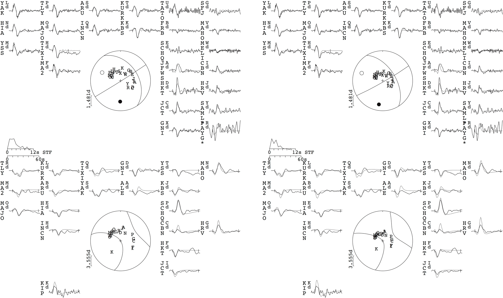
Figure S2. Point-source models for the 2003 Mw 5.9 earthquake. An oceanic structure was used for the left model and a shelf structure for the right model. The best-fitting mechanism for the oceanic structure is a strike of 326°, a dip of 41°, and a rake of 178° at a depth of 16 km and a moment of 1.079×10¹⁸ N·m and for shelf structure is a strike of 328°, a dip of 55°, and a rake of 176° at a depth of 13.5 km and a moment of 8.018×10¹⁷ N·m. P waves are plotted on the top half of the figure for each model, and SH waves are on the bottom half. Seismograms are not normalized, and P wave amplitudes are increased by a factor of five. Station names are to the far left, and the letter to the near left of each seismogram indicates the location on the focal sphere. A star indicates a station that was left out of the inversion.
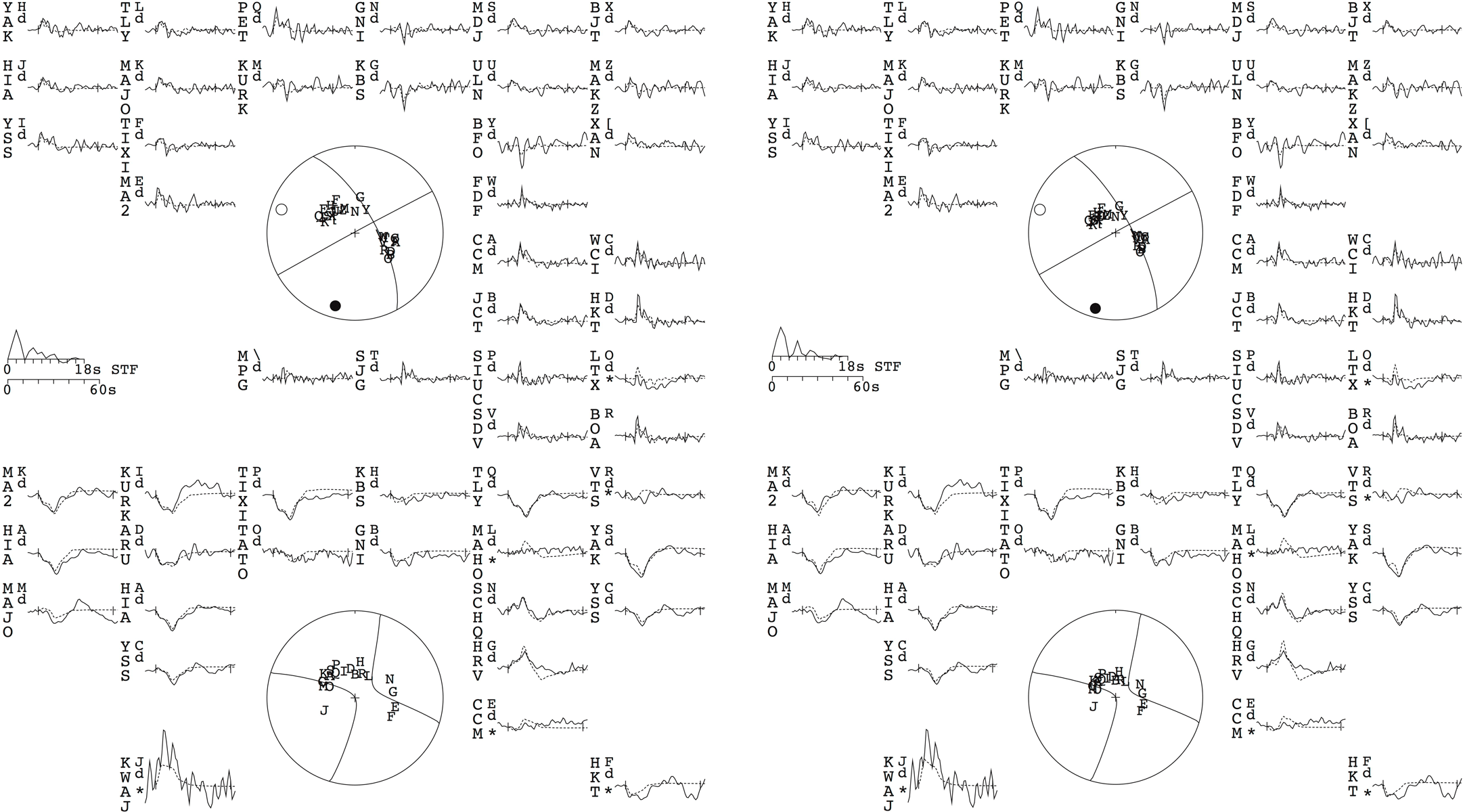
Figure S3. Point-source models for the 2001 Mw 6.2 earthquake. An oceanic structure was used for the left model and a shelf structure for the right model. The best-fitting mechanism for the oceanic structure is a strike of 332°, a dip of 70°, and a rake of 181° at a depth of 16 km and a moment of 1.795×10¹⁸ N·m and for the shelf structure is a strike of 332°, a dip of 75°, and a rake of 181° at a depth of 13 km and a moment of 1.389×10¹⁸ N·m. P waves are plotted on the top half of the figure for each model, and SH waves are on the bottom half. Seismograms are not normalized, and P wave amplitudes are increased by a factor of five. Station names are to the far left, and the letter to the near left of each seismogram indicates the location on the focal sphere.
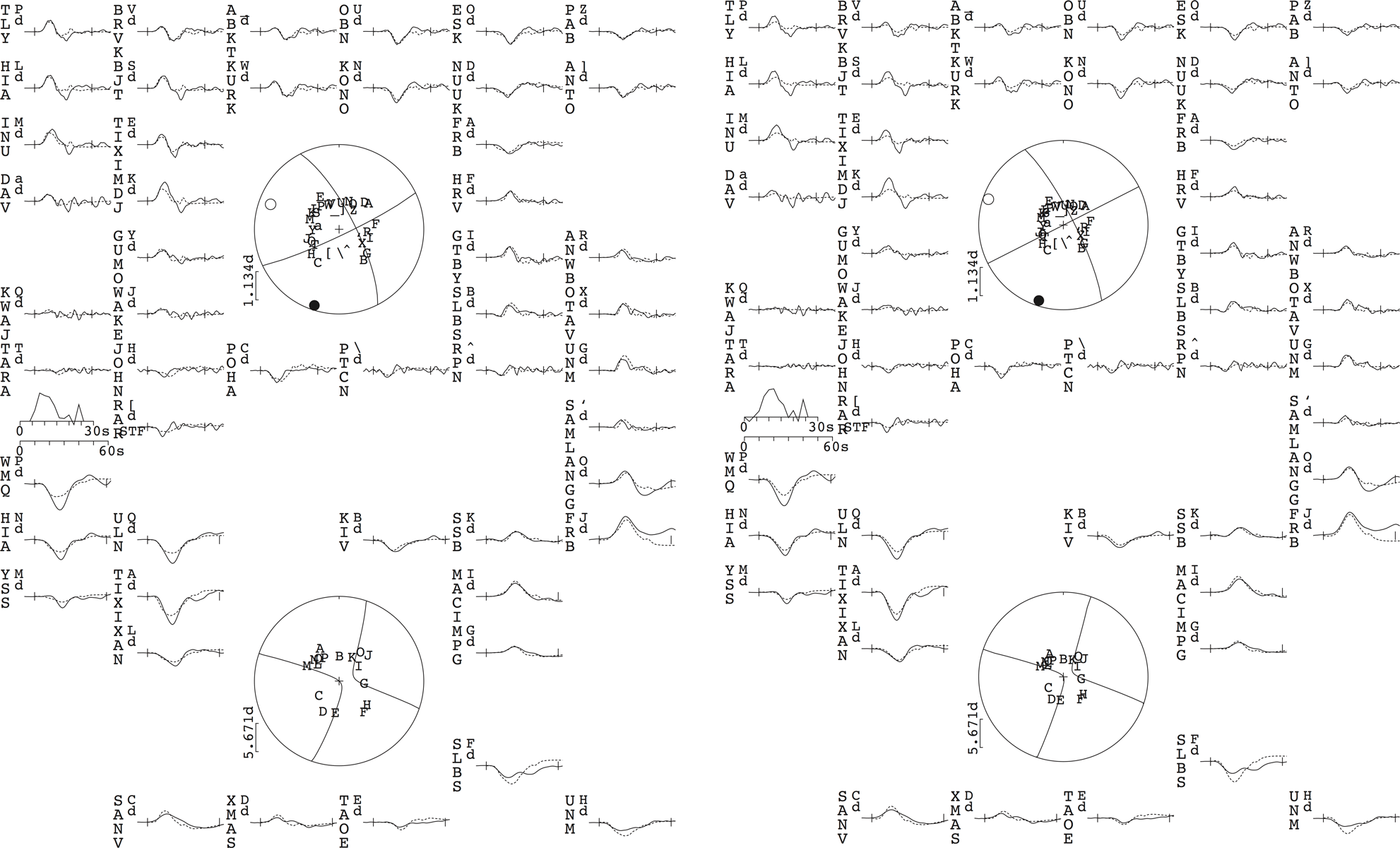
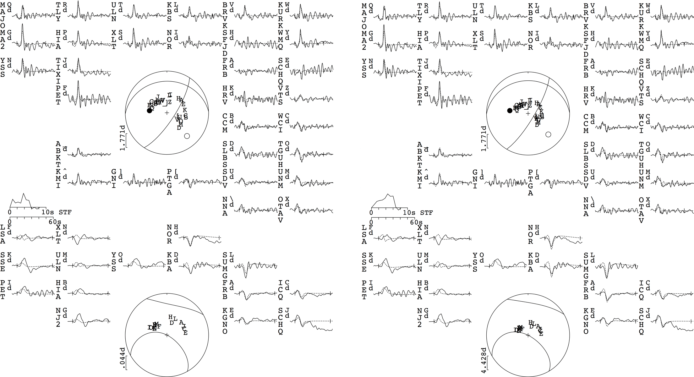
Figure S4. Point-source models for the 2013 Mw 7.5 Craig earthquake. An oceanic structure was used for the left model and a shelf structure for the right model. The best-fitting mechanism for the oceanic structure is a strike of 333°, a dip of 75°, and a rake of 174° at a depth of 18 km and a moment of 2.128×10²⁰ N·m and for the shelf structure is a strike of 333°, a dip of 80°, and a rake of 180° at a depth of 11 km and a moment of 1.549×10²⁰ N·m. P waves are plotted on the top half of the figure for each model, and SH waves are on the bottom half. Seismograms are not normalized, and P wave amplitudes are increased by a factor of five. Station names are to the far left, and the letter to the near left of each seismogram indicates the location on the focal sphere. A star indicates a station that was left out of the inversion.
Figure S5. Point-source models for the 31 January 2013 Mw 5.9 aftershock. An oceanic structure was used on the left and a shelf structure on the right. The best-fitting mechanism for the oceanic structure is a strike of 33°, a dip of 75°, and a rake of 249° at a depth of 7 km and a moment of 9.177×10¹⁷ N·m and for the shelf structure is a strike of 31°, a dip of 78°, and a rake of 251° at a depth of 4 km and a moment of 9.861×10¹⁷ N·m. P waves are plotted on the top half of the figure for each model, and SH waves are on the bottom half. Seismograms are not normalized, and P wave amplitudes are increased by a factor of five. Station names are to the far left, and the letter to the near left of each seismogram indicates the location on the focal sphere.
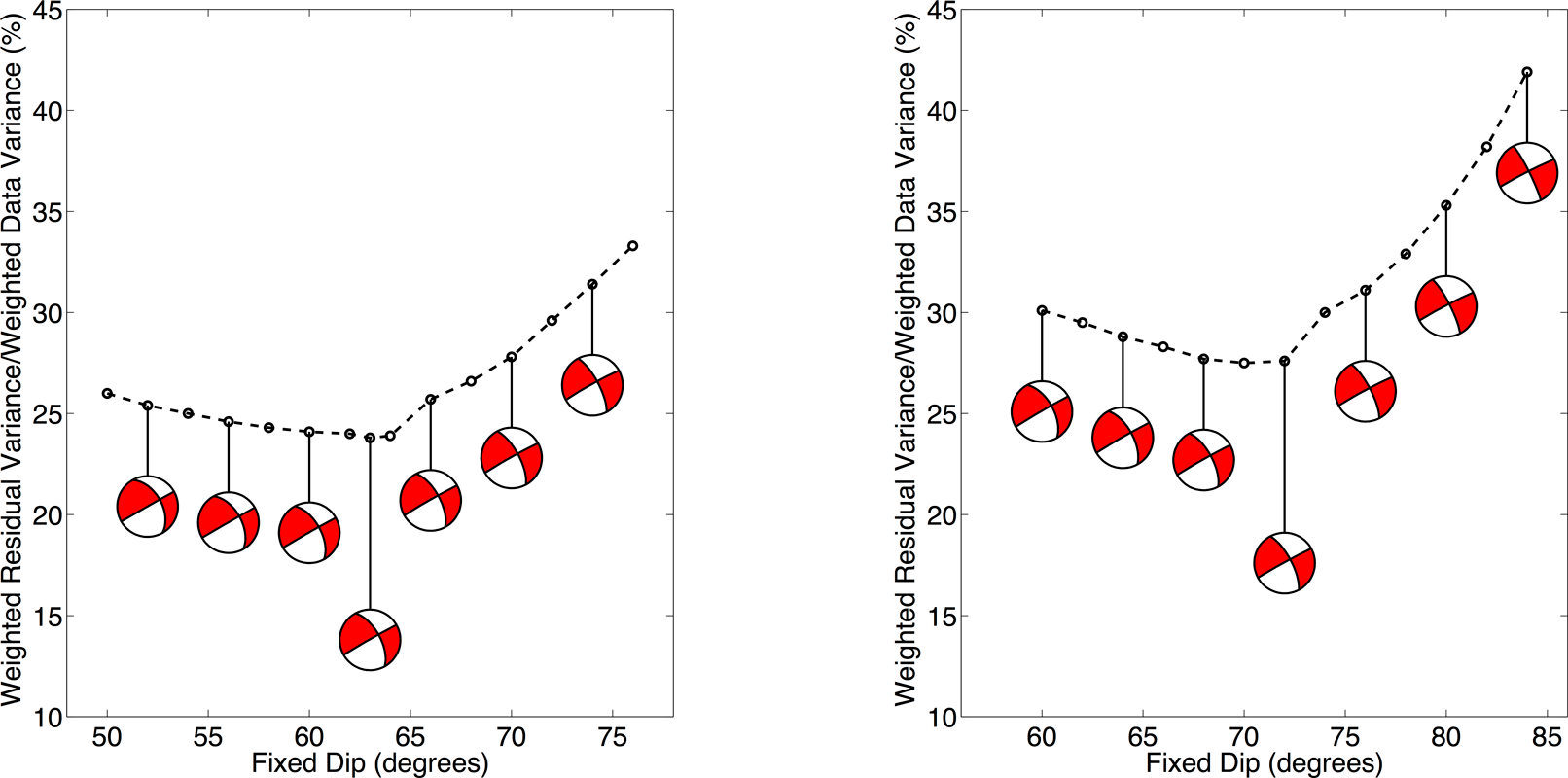
Figure S6. Dip sensitivity testing for the 2004 Mw 6.8 earthquake. An oceanic structure is used on the left and a shelf structure on the right. Dips were fixed at 2° increments with all other parameters left free. Best-fitting mechanisms are shown every 4°, and the best mechanism with all parameters left free is plotted in the center. Note how the steeper dips are constrained by the stations to the east of this earthquake, with relatively few stations to the west to constrain the shallower dips.
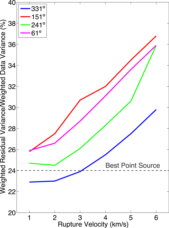
Figure S7. Directivity testing for the 2004 Mw 6.8 earthquake. An oceanic structure was used, but results were similar for a shelf structure. The variance reduction for the best point source is shown in a grey dashed line. Rupture velocities of 1–6 km/s were tested in each of the directions determined from 90° increments of the strike of the best point source mechanism. Rupture velocities of 1–3 km/s in the 331° strike direction had higher variance reductions than the point source. This would be consistent with rupture along the Queen Charlotte–Fairweather fault in the northwest direction, similar to the 2013 Craig earthquake.
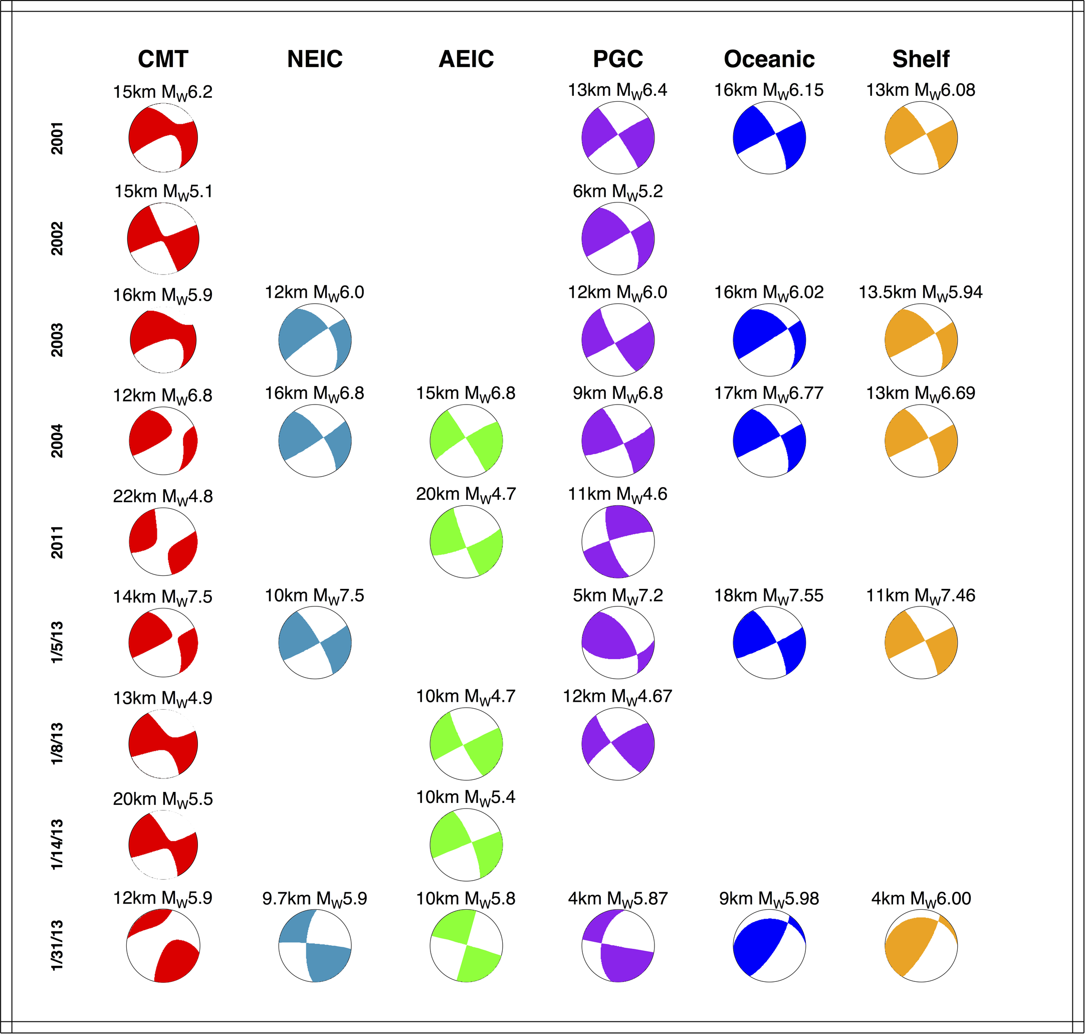
Figure S8. Reference for moment tensors and focal mechanisms. All available mechanisms for the earthquakes in this study: (from left to right) moment tensors from the Global CMT catalog, focal mechanisms from the NEIC, best double couple of AEIC regional moment tensors, best double couple of PGC regional moment tensors, and best fit point source solution from this study in oceanic structure and in shelf structure.
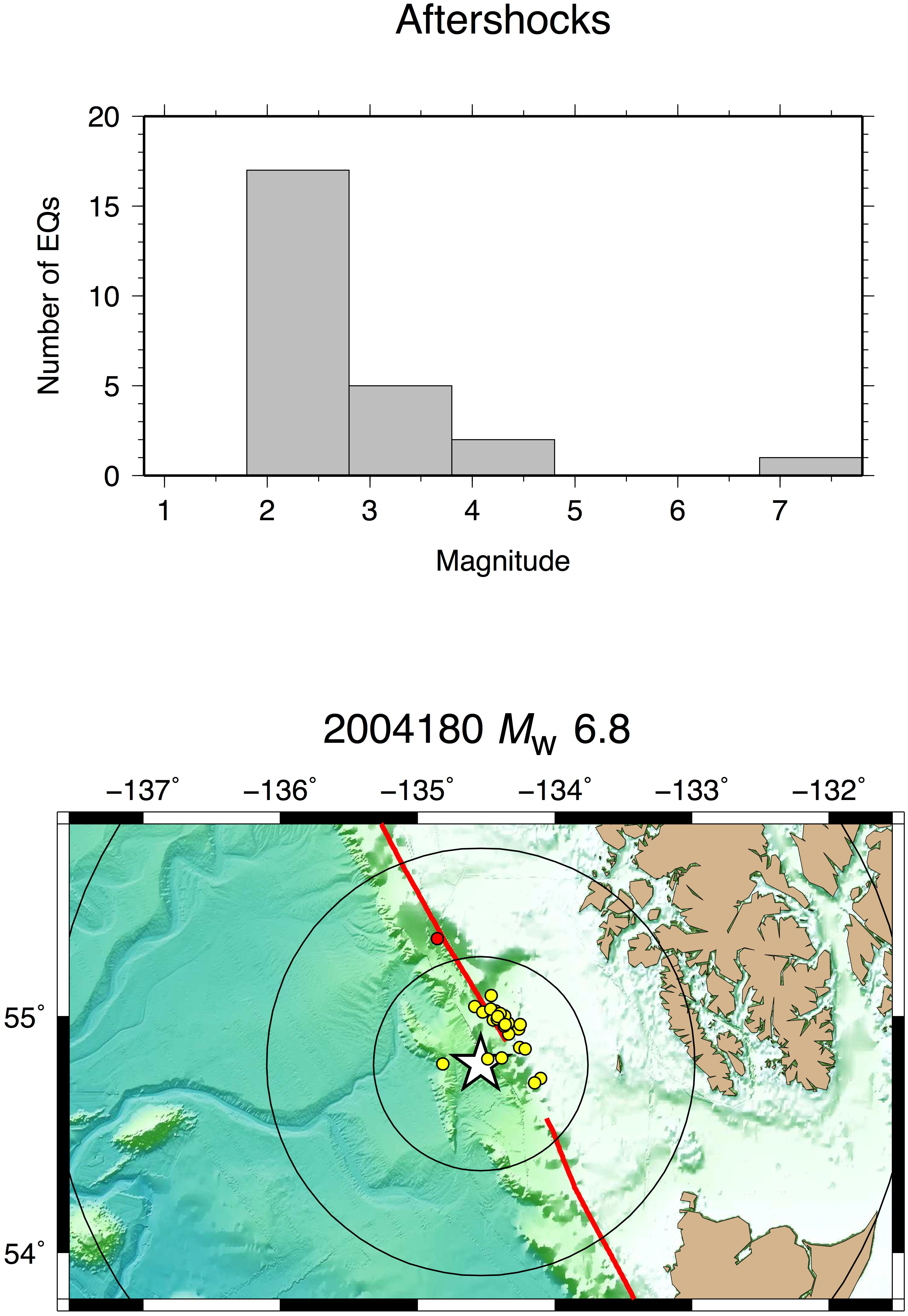
Figure S9. Aftershocks for the 2004 Mw 6.8 earthquake. The histogram at the top shows the magnitude distribution, and the bathymetry map at the bottom shows the spatial distribution of aftershocks, plotted as yellow circles. Red lines denote mapped faults. The NEIC hypocenter of the earthquake is plotted as a white star, and the black circles show 50, 100, and 200 km radius from the hypocenter. The red circle is the one earthquake that occurred before the mainshock.
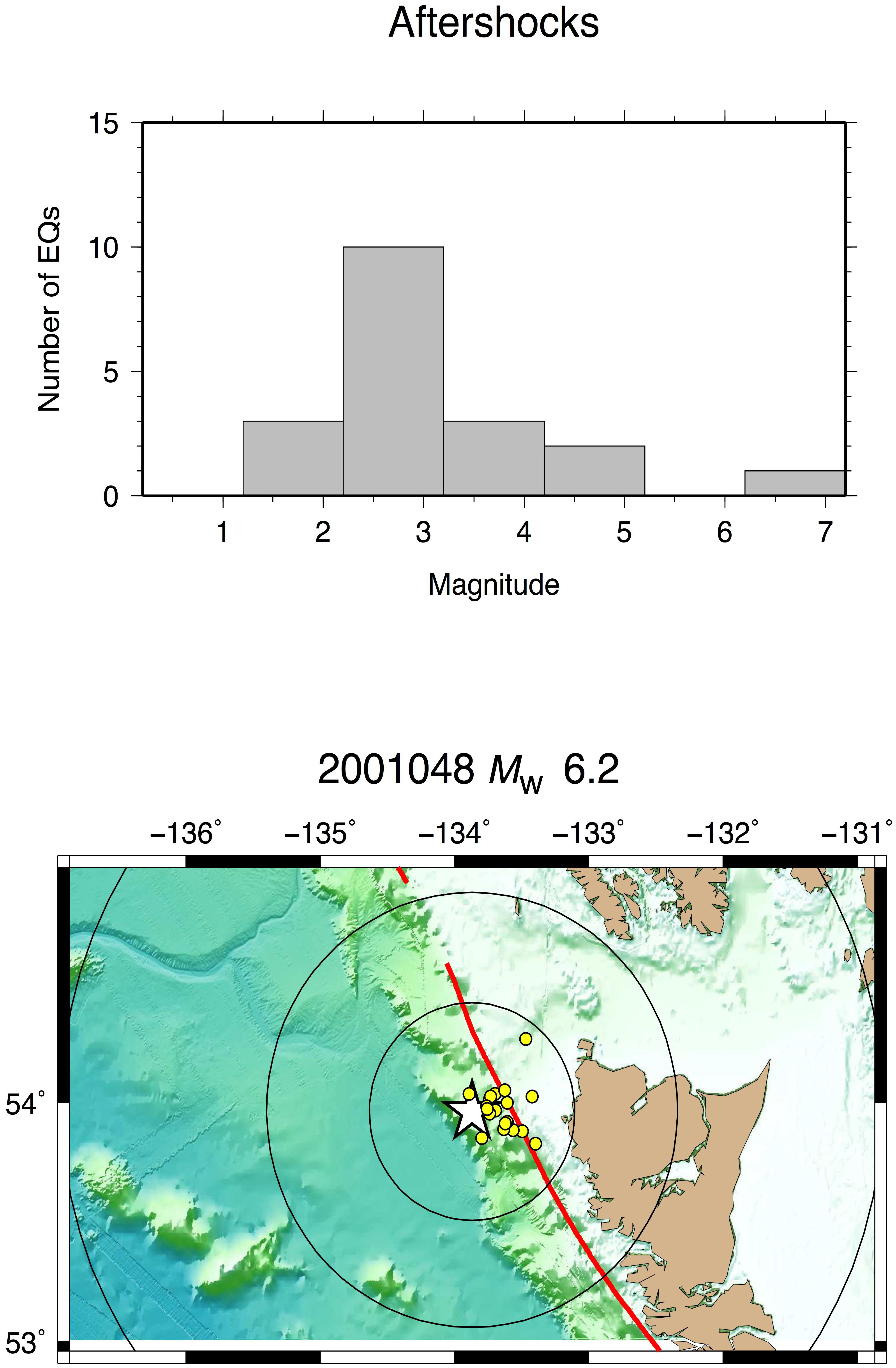
Figure S10. Aftershocks for the 2001 Mw 6.2 earthquake. The histogram at the top shows the magnitude distribution, and the bathymetry map at the bottom shows the spatial distribution of aftershocks, plotted as yellow circles. Red lines denote mapped faults. The NEIC hypocenter of the earthquake is plotted as a white star, and the black circles show 50, 100, and 200 km radius from the hypocenter.
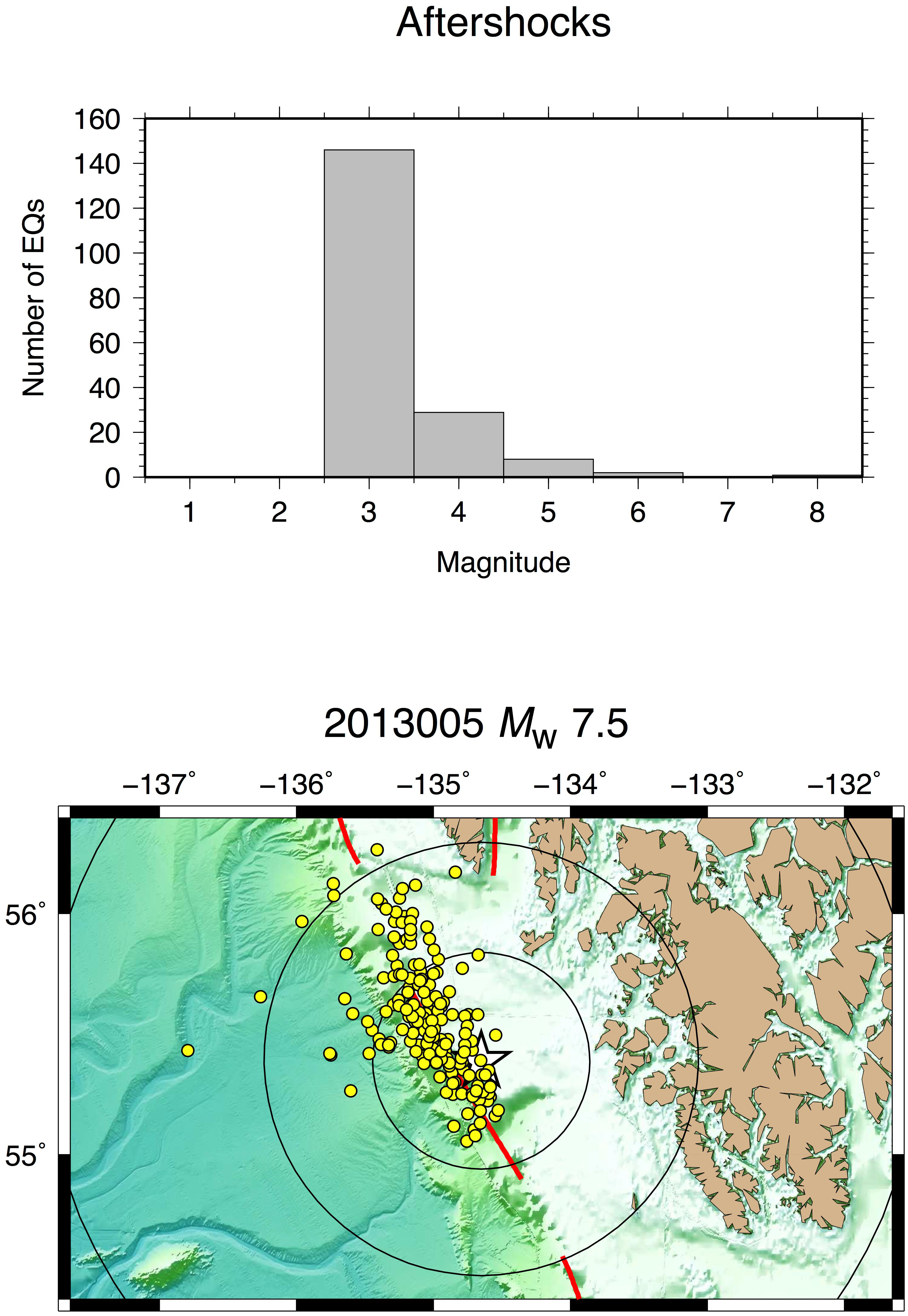
Figure S11. Aftershocks for the 2013 Mw 7.5 Craig earthquake. The histogram at the top shows the magnitude distribution, and the bathymetry map at the bottom shows the spatial distribution of aftershocks, plotted as yellow circles. Red lines denote mapped faults. The NEIC hypocenter of the earthquake is plotted as a white star, and the black circles show 50, 100, and 200 km radius from the hypocenter.
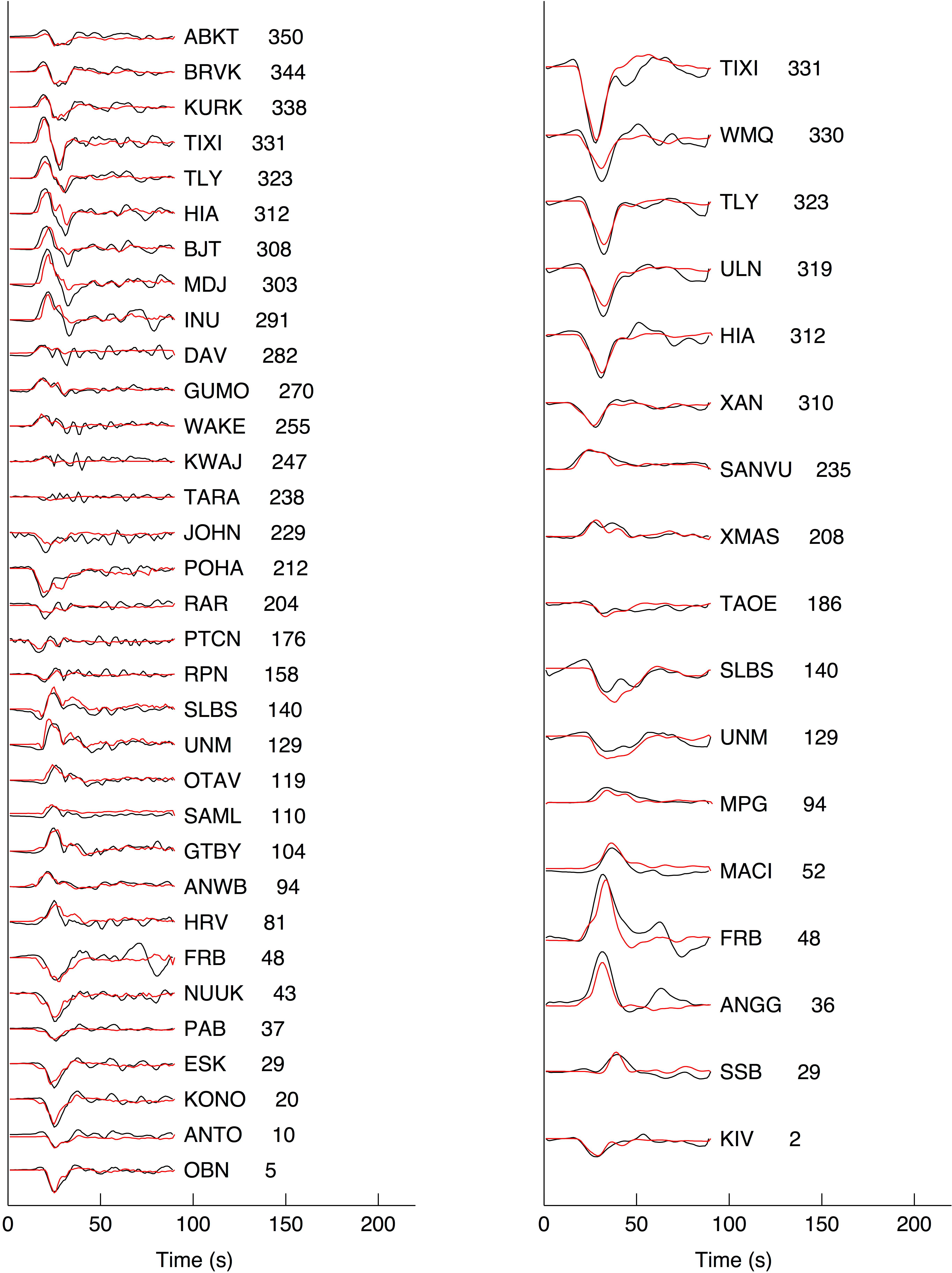
Figure S12. Stations used in the finite-fault slip inversion of the 2013 Craig earthquake. The seismograms show P waves (left) and SH waves (right), with black for the recorded data and red for the calculated synthetics. A sedimentary structure is used for the source velocity. These synthetics are for the full fault model of 300 km in length, 0–50 km in depth, and a dip of 75°, with the rupture velocity of 4 km/s at the 333° strike and 1 km/s in the opposite 153° direction. The hypocenter begins at 15 km in depth and is centered at the change in rupture velocity.
[ Back ]