This electronic supplement contains additional description and figures showing estimated source amplitudes obtained with different parameters and observed amplitudes of some earthquakes with large misfits.
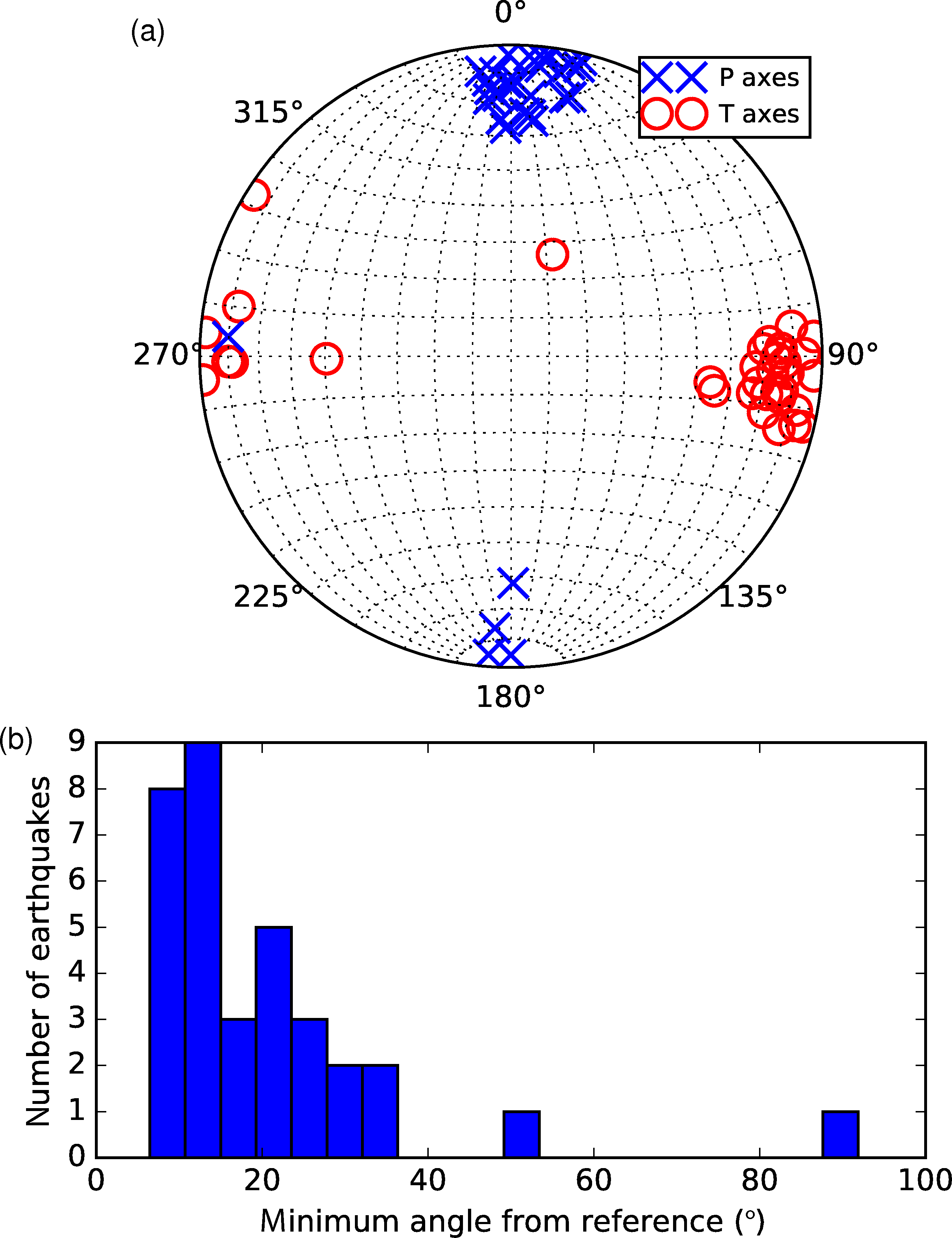
In our analysis, we assume that closely spaced earthquakes have the same focal mechanisms. To test this assumption, in Figure S1a we plot the pressure and tension axes of the 34 Mw >3.1 earthquakes located in the study area, which have reviewed the focal mechanisms in the Northern California Seismic Network (NCSN) catalog. All but two are consistent with right-lateral slip on the northwest-trending San Andreas fault. We compare these focal mechanisms with a reference focal mechanism suggested by the seismicity distribution, which defines a plane that strikes 135° and dips 80° to the southwest. Figure S1b shows the distribution of minimum rotation angles to move the observed focal mechanism to the focal mechanism representing horizontal slip on the seismicity-defined fault plane (compute as in Kagan, 2007). Most of the rotation angles are smaller than 30°, implying that the focal mechanisms are roughly the same, and it is appropriate to assume that most earthquakes in our study area have the same focal mechanisms.
However, there clearly is some variation in the observed focal mechanisms, and there could be more variation for smaller earthquakes. Such variation in focal mechanism could give rise to variations in the seismic amplitude, especially for observations near the nodal planes, where amplitude varies strongly with azimuth. To check that the focal mechanisms are not playing a major role in our source amplitude estimates, we weight the observations to include information from a range of azimuths, and we redo our inversions without data near the nodal planes, where we expect focal mechanism variability to have the largest effect. Both of these assessments are described in the Weighting by Azimuth section.
As described in the Obtaining Relative Source Amplitudes section, we input the observed log spectral amplitudes into the system of equation (5) in the main article to solve for the log amplitudes of the sources. This set of equations is
cijk(si − sk) = cijk(dik − djk).
The solution to this set of equations depends on how strongly each equation contributes. We exclude some of the equations and modify the weightings cijk to improve the robustness of the source amplitude estimates.
First, to maintain more robust results, we consider only earthquake pairs that have multiple observations of their ratios. We use an observation dik − djk only if there are at least five stations k. Second, we exclude groups of earthquakes that do not have a large number of links to the main event. As an extreme example, consider the small cluster of earthquakes at 16 km depth and 10 km along-strike distance in Figure 9 of the main article. These earthquakes likely have similar Green’s functions, so we can compare the source amplitudes within this cluster by comparing the observed seismic amplitudes, but we have no way to eliminate their Green’s functions for comparison with the remaining shallower events. To exclude the earthquakes that are poorly tied to the main group, we split the events into half-kilometer boxes according to their location along strike and with depth. For each pair of boxes, we count the number of amplitude ratio observations where one earthquake is in each box. Two boxes are linked if at least 20 observations tie them together. Earthquakes in boxes that are not linked into the main group are excluded.
Next, we choose the weightings cijk. One plausible weighting specifies that each observation of a log spectral amplitude dik contributes equally. However, the data dik − djk on the right side of equation (1) in the main article are differences in log spectral amplitudes. If this system of equations is solved without weighting (if each cijk = 1), individual observations will be weighted unequally. As one example, imagine that station 1 records 10 earthquakes, whereas station 2 records 20. Station 1 then provides 45 pairs of observations—45 dik − djk—whereas station 2 provides 190. In this case, a unit squared error at station 2 would contribute roughly four times as much to the misfit as a unit squared error at station 1: approximately (190/20)2 as opposed to (45/10)2. To alleviate this variable weighting, we weight the misfit from the amplitude ratio dik − djk by (nik njk)−1/2. (Each cijk scales as (niknjk)1/4.) This weighting roughly equalizes the importance of each observation.
On the other hand, it is not clear that each observation of an amplitude contains independent information. The spectral amplitude ratio between pairs of earthquakes often varies between stations. These changes in amplitudes are probably not due to noise, but to variations in local structure or focal mechanisms. Such variations could depend on azimuth. Azimuthal variations are especially problematic because stations in California are concentrated along the San Andreas fault, to the northwest and southeast of the earthquakes considered here.
To address this variation, we first add a weighting to equation (5) in the main article that allows for a more constant azimuthal dependence. We compute the number of observations (dik, not dik − djk) as a function of azimuth. We smooth this histogram with a Gaussian with half-width 20° and use it to reweight the observations. If w(ϕ) is the smoothed number of observations as a function of azimuth ϕ, the weights in equation (5) in the main article are cijk = (nik−1/2 njk−1/2 w(ϕ)−1)1/2.
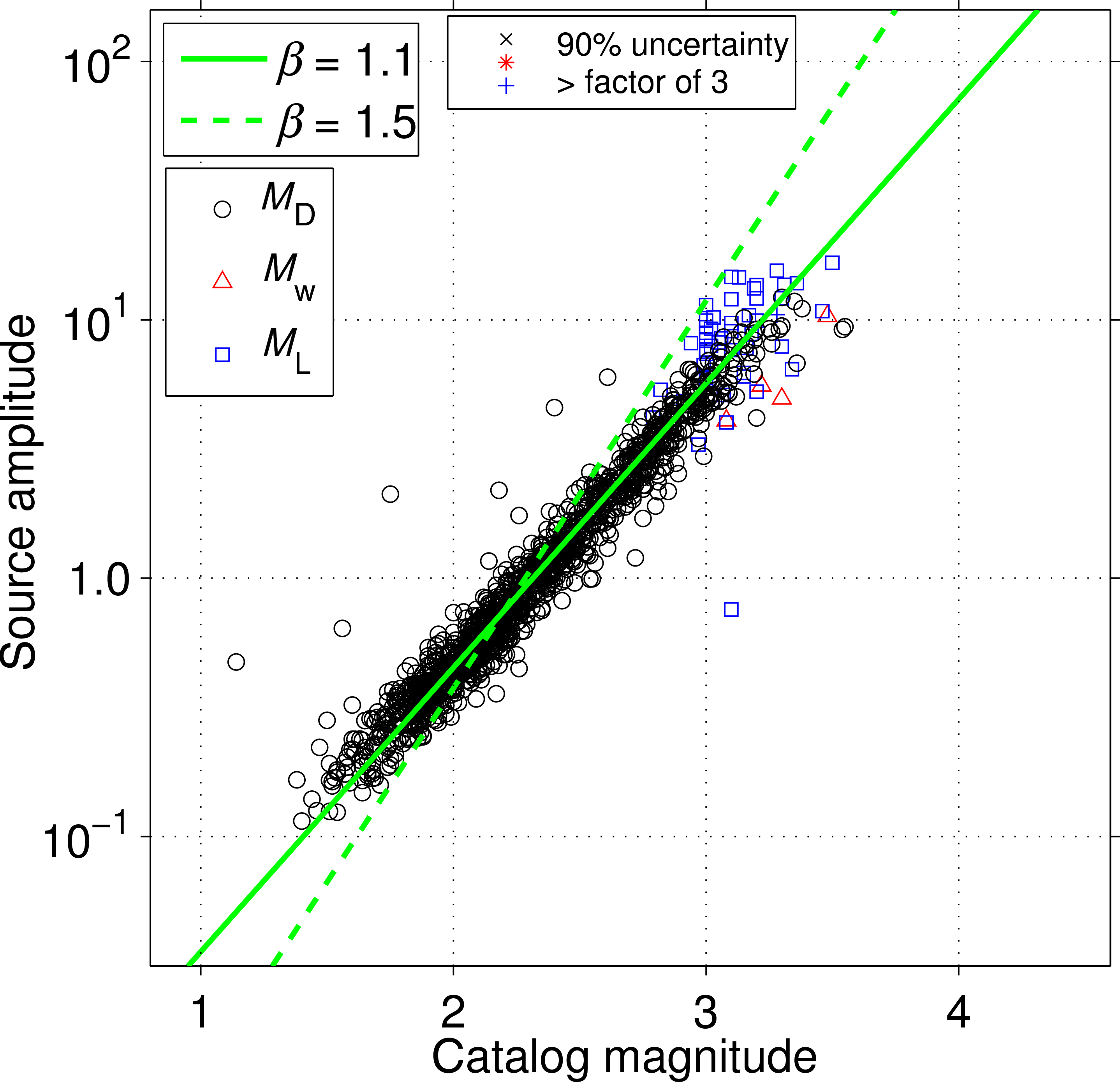
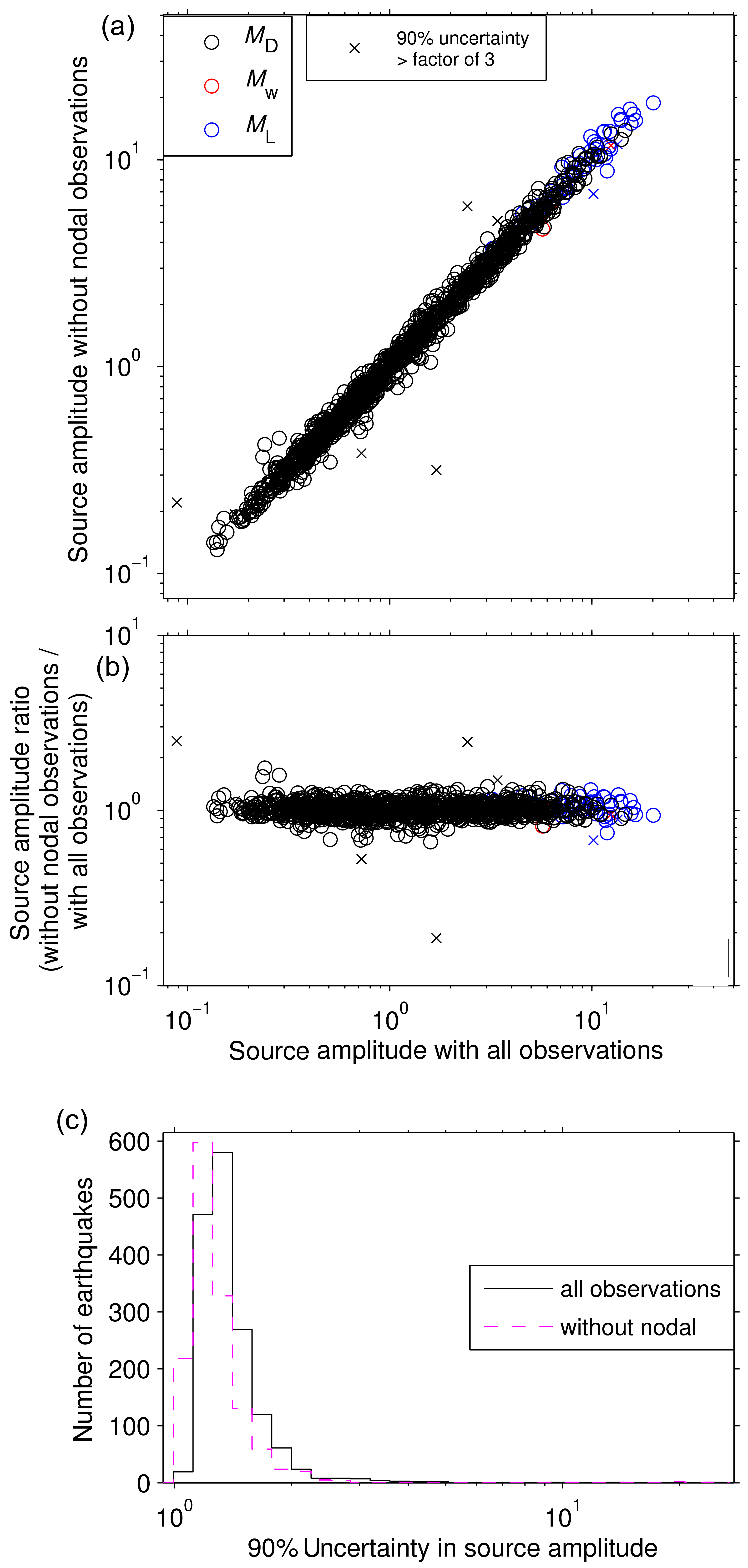
Uncertainty in the appropriate azimuthal weighting is problematic because there could be a bias in focal mechanisms between large and small earthquakes. Larger earthquakes may be more likely to occur on the fault plane. They may therefore have more consistent focal mechanisms than the smaller earthquakes, and the uneven azimuthal distribution of stations could bias our results. To look for this bias, we perform an inversion without data near the expected nodal planes. We exclude all data with earthquake-station azimuths within 15° of 135°, 225°, 315°, or 45°. The resulting moment-magnitude plot is shown in Figure S2. Within the uncertainty, it gives the same scaling parameters as the original results. In Figure S3a, we plot the earthquake source amplitudes obtained with and without the nodal observations. 90% of the amplitude ratios with the two schemes are between 0.84 and 1.13, well within the bootstrap estimates. The bootstrap error estimates are slightly smaller when we exclude the nodal observations. The median 90% uncertainties are a factor of 1.32 with all observations and 1.23 without the nodal observations (see Fig. S3c).
A final concern in our inversion is that some observations could contribute especially strongly and bias our results. We alleviate this problem in two ways. First, we compute the weighting for each observation (again dik, not dik − djk), and we throw away any observations that have weightings more than four standard deviations different than the median weighting. Second, we use an absolute value norm for large misfits. When the (unweighted) difference between the observed and predicted log spectral ratios is smaller than 0.3, the misfit is computed with a least-squares norm. When it is larger, the misfit is computed with an absolute value norm. This misfit calculation makes our system of equations less dependent on individual observations with large misfit.
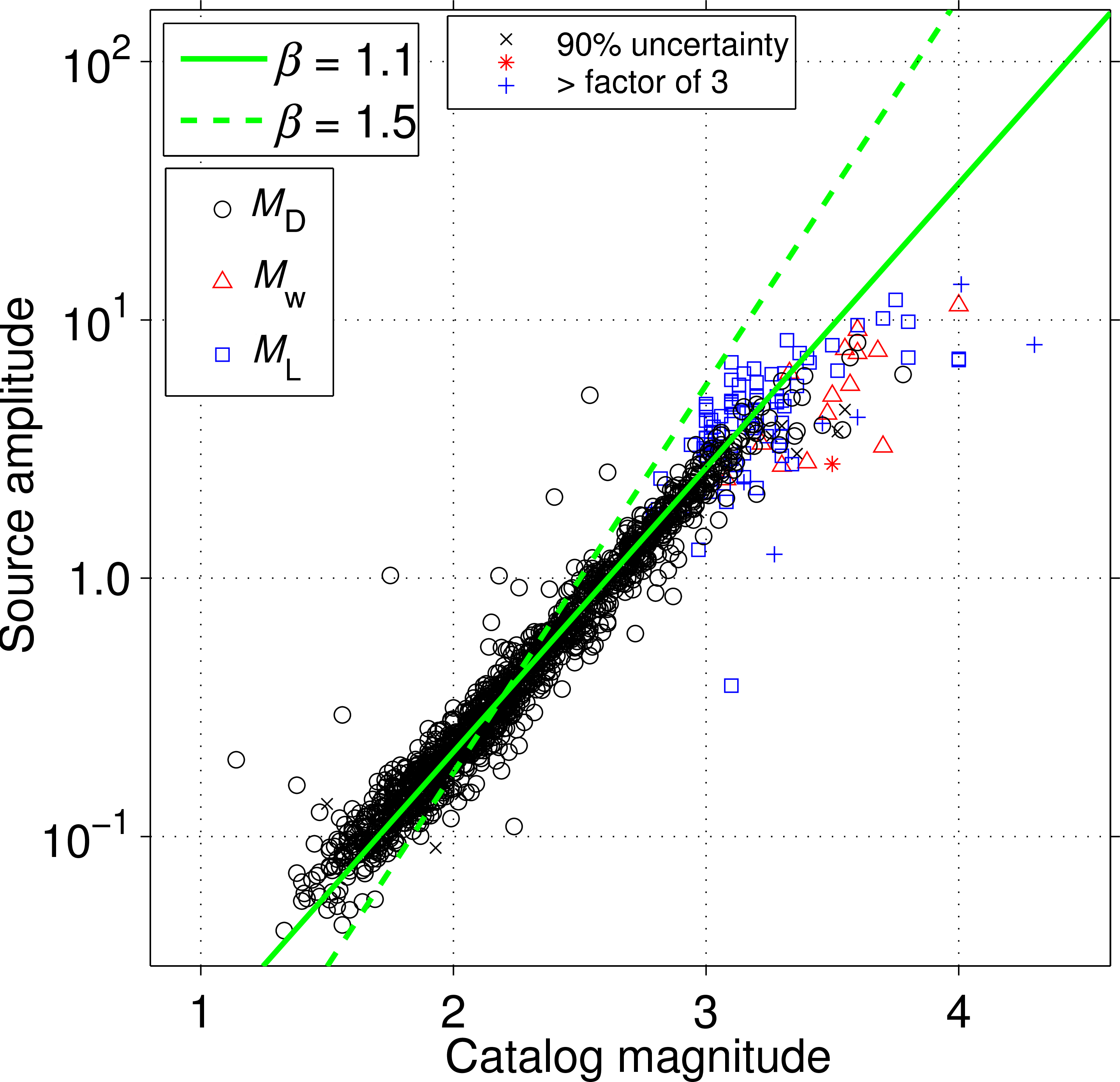
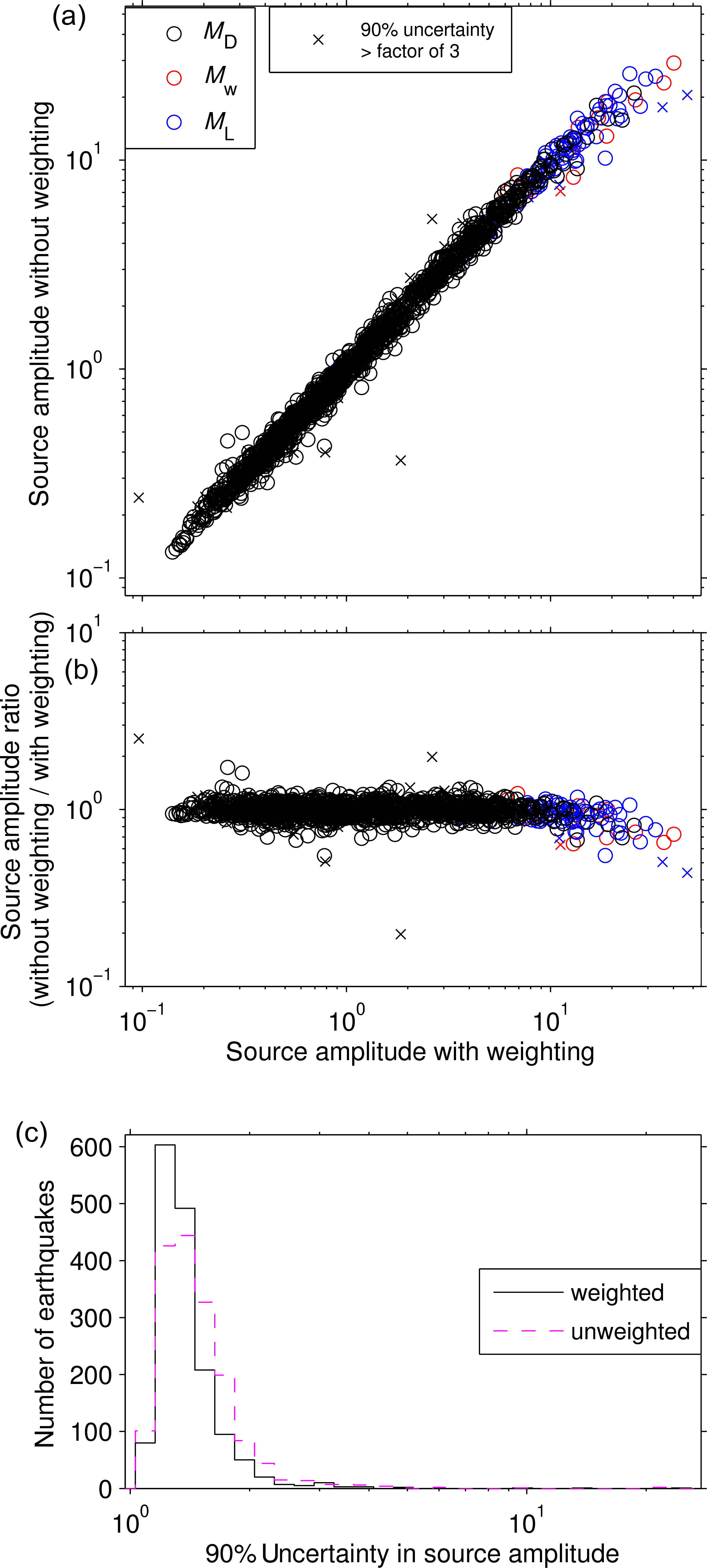
To assess the importance of the preferred weighting scheme, we compare the results obtained with and without the weights. Figure S4 shows the source amplitudes obtained when we weight each ratio equally, so that all cijk are set to 1. We obtain nearly the same magnitude scaling, with a best-fitting β of 1.11 and 90% of the bootstrapped estimates between 1.09 and 1.15. When we directly compare the estimated source amplitudes obtained with the two weighting schemes, 90% of the amplitudes are within a factor of 0.88–1.18 of each other, as shown in Figure S5b. The bootstrap uncertainties are slightly larger without the preferred weighting, giving a median 90% uncertainty of a factor of 1.41 rather than 1.32 (Fig. S5c), though these uncertainties do not fully describe the potential errors. Because earthquake source amplitudes are linked by observations, amplitudes of groups of events can be systematically offset but still within the bootstrap errors, as seen for some of the larger earthquakes in Figure S5b. The consistency between the inversions with and without our preferred weighting suggest that for the earthquakes considered, the data are consistent and abundant enough that the improved source amplitudes obtained with the weighting are modest.
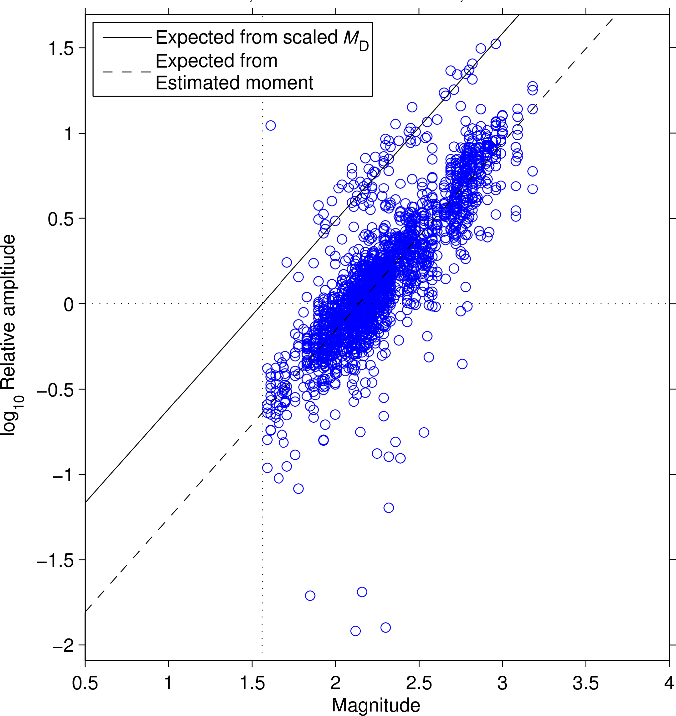
In the Scaling to Moment and Catalog Magnitude section, we saw that several earthquakes had estimated moments that differed significantly, by more than a factor of 3, from the moments expected from the magnitude calibration even though the bootstrap uncertainties are reasonably low. We also estimated the moment of one event with poorly determined magnitude cataloged as an Mh 0 earthquake (Fig. S15). In Figures S6–S15, we compare the amplitudes of these 10 earthquakes with those of other events within 2 km. Each point shows the amplitude ratio obtained for a single station, the amplitude of a nearby earthquake compared with that of the earthquake of interest. Though there are a few errors that could be associated with incorrect gain corrections, the individual amplitude ratios mostly reflect the moment obtained from the inversion (dashed lines). Only one (Fig. S6) shows any systematic misfit from the inversion results and the individual amplitudes.
The 4-second amplitudes we use in the inversion are also reflected in visual examination of the amplitude of the P-wave arrivals in the waveforms. Most of the earthquakes with large misfits are followed by cataloged events within 6–30 s. However, all of the later events occur within 4 km of the original event and thus should show similar arrival times. We do not observe arrivals from other earthquakes that would clearly contaminate the records.
The earthquakes with large misfits do not appear to occur in a particular time or place, making it hard to explain the amplitude differences with errors in gain corrections. Other earthquakes occurring with 1 day of the outlier events do not have unexpected moment estimates. For 44 out of 49 earthquakes, the log10 misfits are smaller than 0.1. We have reproduced the amplitude differences using a different code for obtaining the data and correcting for response, with ObsPy (Beyreuther et al., 2010), and obtained similar relative amplitudes. It remains unclear to us why our moments differ strongly from the catalog magnitude estimates for this handful of events.
Figure S1. (a) Pressure and tension axes of the 34 earthquakes in the study area, which have reviewed the focal mechanisms in the NCSN catalog. (b) Minimum rotation angle between these focal mechanisms and the reference focal mechanism suggested by the distribution of seismicity.
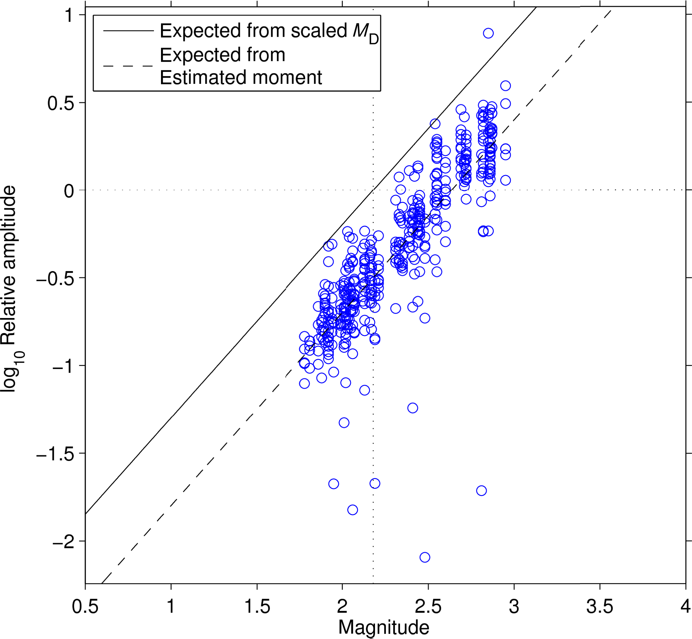
Figure S2. Estimated relative amplitudes versus catalog magnitude as in Figure 3 of the main article. These amplitudes are computed without data from stations within 15° of the strike of the San Andreas. Note that these amplitudes are not adjusted for corner frequency.
Figure S3. (a) Source amplitudes estimated without (y axis) and with (x axis) the nodal observations. (b) Ratio of source amplitudes obtained without the nodal observations to those obtained with all observations. (c) Distribution of 90% bootstrap errors with all observations (solid line) and excluding the nodal observations (dashed line).
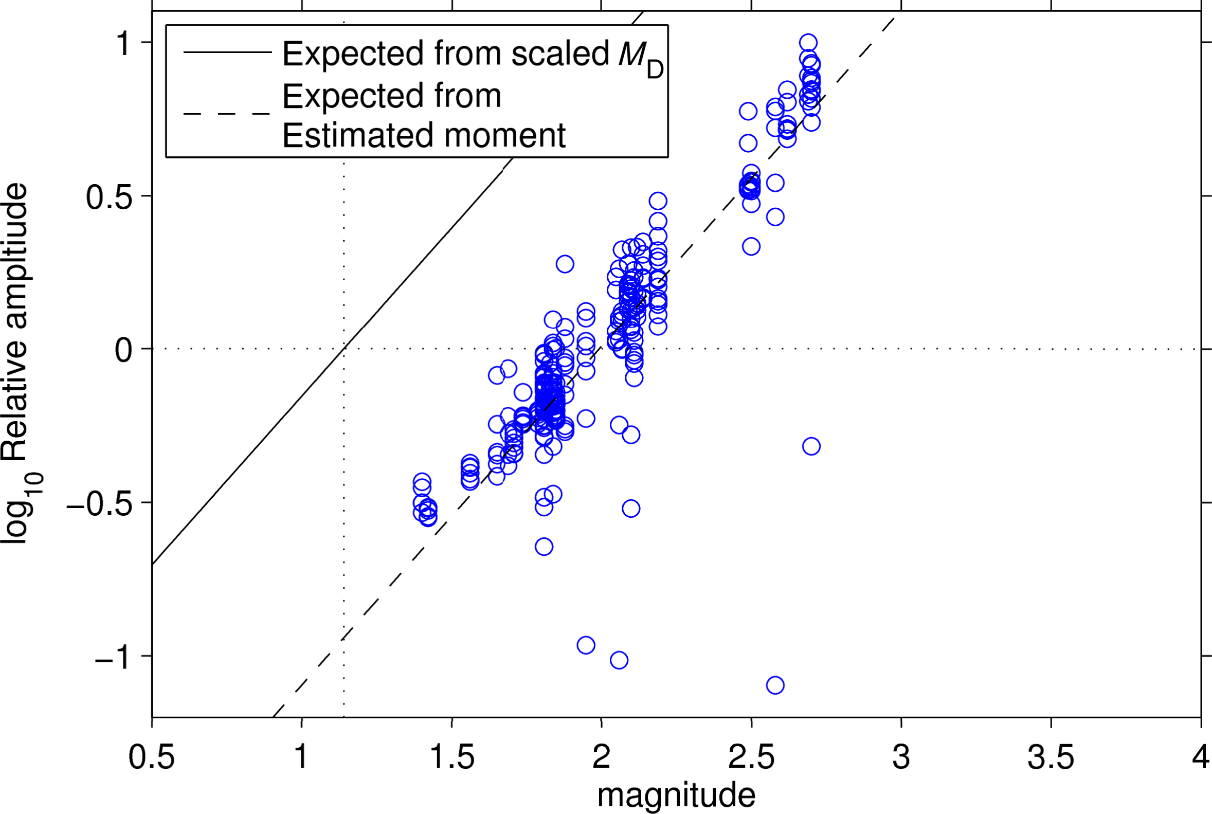
Figure S4. Estimated relative amplitudes versus catalog magnitude as in Figure 7 of the main article. These amplitudes are computed without any weighting adjustments for the number of observations or azimuthal distributions. Each ratio is weighted equally.
Figure S5. (a) Source amplitudes estimated without (y axis) and with (x axis) weights adjusted for the number of observations and their azimuthal distribution. (b) Ratio of source amplitudes obtained without the adjusted weights to those obtained with the preferred weights. (c) Distribution of 90% bootstrap errors with the preferred weights (solid line) and with equal weight per ratio (dashed line).
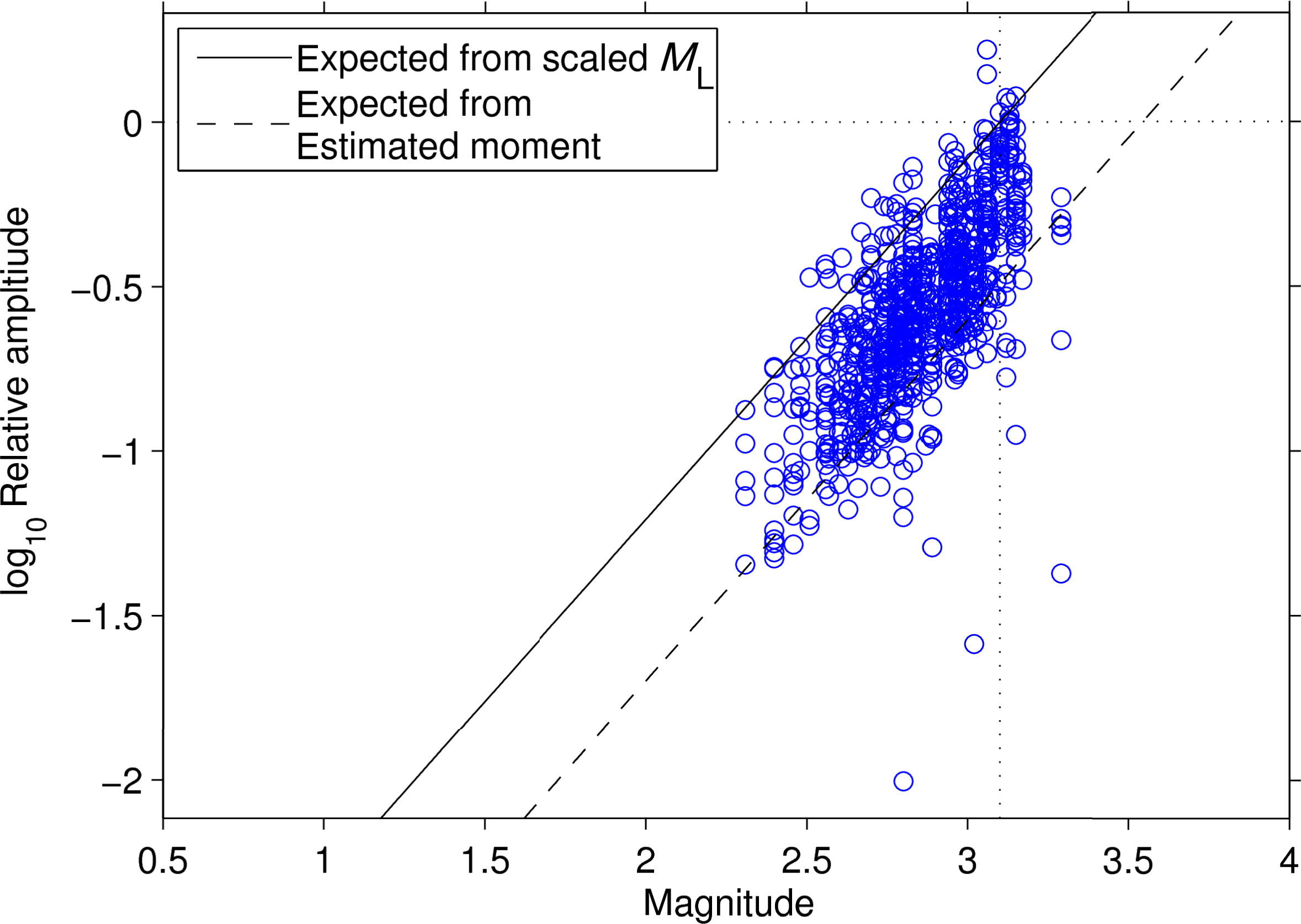
Figure S6. Seismogram amplitudes of nearby earthquakes divided by that of an ML 3.1 earthquake (NCSN id: 116946) on 10 May 1988, 12:31:31. The solid line shows the prediction from the magnitude scaling calibration, whereas the dashed line adjusts that prediction for the estimated moment of the ML 3.1 earthquake.
Figure S7. As in Figure S6, but for an MD 0.8 earthquake (NCSN id: 159528) on 15 June 1990, 20:25:33.
Figure S8. As in Figure S6, but for an ML 3.1 earthquake (NCSN id: 203850) on 31 December 1990, 13:33:24.
Figure S9. As in Figure S6, but for an MD 1.6 earthquake (NCSN id: 30075599) on 25 June 1995, 15:04:31.
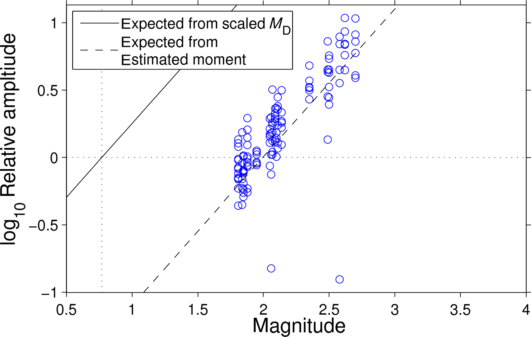
Figure S10. As in Figure S6, but for an MD 2.6 earthquake (NCSN id: 559226) on 4 March 1998, 06:01:00.
Figure S11. As in Figure S6, but for an MD 2.4 earthquake (NCSN id: 561959) on 15 March 1998, 06:50:29.
Figure S12. As in Figure S6, but for an MD 2.2 earthquake (NCSN id: 30192544) on 12 August 1998, 14:24:08.
Figure S13. As in Figure S6, but for an MD 1.1 earthquake (NCSN id: 30191621) on 17 August 1998, 00:36:47.
Figure S14. As in Figure S6, but for an MD 1.8 earthquake (NCSN id: 30214173) on 18 January 1999, 00:16:20.
Figure S15. As in Figure S6, but for an event with poorly determined catalog magnitude, cataloged as Mh 0.0 (NCSN id: 51184156) on 15 July 2007, 21:57:10.
We used seismic waveform data and the Northern California Seismic Network (NCSN, http://www.ncedc.org/) earthquake catalog, provided by the Northern California Earthquake Data Center (NCEDC) and the Berkeley Seismological Laboratory (doi: 10.7932/NCEDC).
Beyreuther, M., R. Barsch, L. Krischer, T. Megies, Y. Behr, and J. Wassermann (2010). ObsPy: A Python toolbox for seismology, Seismol. Res. Lett. 81, no. 3, 530–533, doi: 10.1785/gssrl.81.3.530.
Kagan, Y. Y. (2007). Simplified algorithms for calculating double-couple rotation, Geophys. J. Int. 171, no. 1, 411–418, doi: 10.1111/j.1365-246X.2007.03538.x.
[ Back ]