This electronic supplement contains Figures S1–S15 showing seismic spectra, noise, seismograms, and duration estimates.
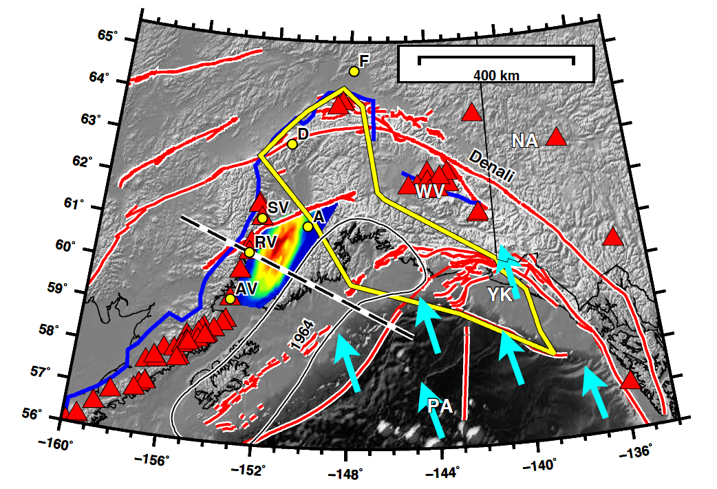
Figure S1. Active tectonic setting of the Aleutian-Alaskan subduction zone, south-central Alaska, and relationship to proposed imaging targets. Triangles denote active volcanoes, including the Wrangell volcanic (WV) field; the lateral extent of deep intraslab seismicity is plotted as a thick line behind the arc. Circles: AV, Augustine Volcano; RV, Redoubt Volcano; SV, Spurr Volcano; A, Anchorage; D, Denali; F, Fairbanks. Southwest of Anchorage is the basement surface of Cook Inlet basin, with a maximal depth of 7.6 km near the center, colored red (Shellenbaum et al., 2010). Plate labels: NA, North America; PA, Pacific; YK, Yakutat block; arrows indicate PA motion relative to NA. Yellow outline denotes the (minimum) subsurface extent of Yakutat slab (Eberhart-Phillips et al., 2006). Blue line marks the lateral extent of deep intraslab seismicity (e.g., Wang and Tape, 2014). Black outline marks the aftershock zone of the 1964 Mw 9.2 earthquake. The thick dashed line denotes the target 2D subduction profile in this study; the Cook Inlet region (slab, crust, basin) is the primary 3D target in this study.
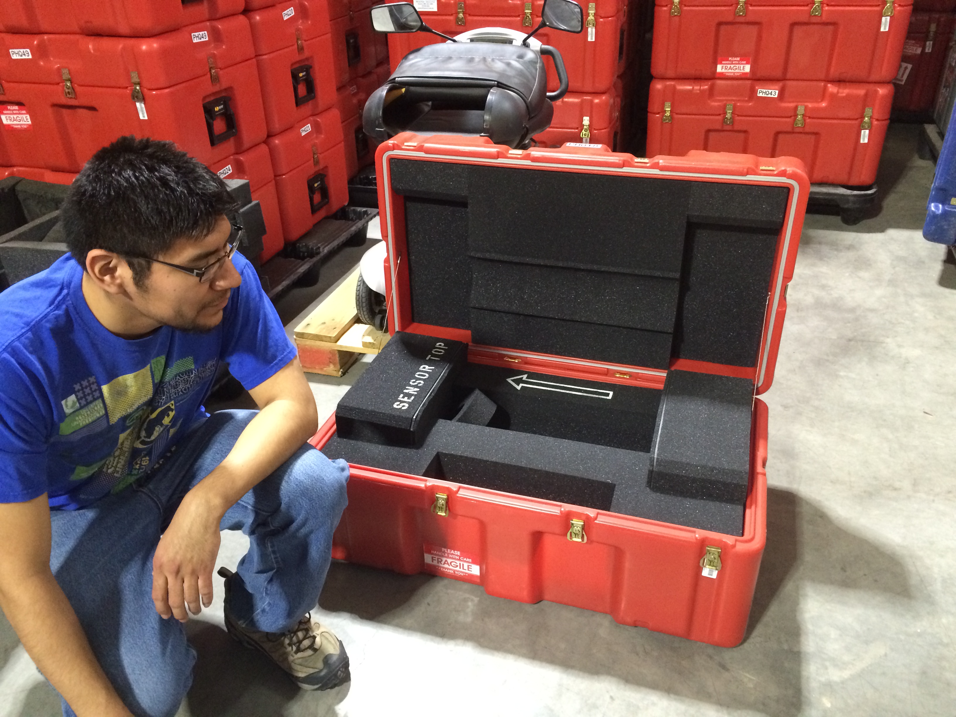
Figure S2. Example of the sensor shipping case used by Incorporated Research Institutions for Seismology (IRIS)/Program for the Array Seismic Studies of the Continental Lithosphere (PASSCAL) for the Nanometrics Trillium T120PH sensors (Kyle Smith for scale). PASSCAL worked with Nanometrics and one of the leading manufacturers of reusable shipping and carrying cases, Pelican, to develop the seismic sensor shipping case. At least three sensors within the initial shipment of 10 were damaged after being shipped from PASSCAL (Socorro, New Mexico) to the University of Alaska Fairbanks (UAF) Marine Science Center in Seward, Alaska. The cases were stacked and wrapped on pallets for shipment. No visible damage to the shipment was apparent, but performance during the huddle test in Seward (Fig. S3) revealed problems that were not present during testing at PASSCAL prior to shipment. (In one case, the mass positions did not center.) Our inference is that the sensors were damaged during shipping.
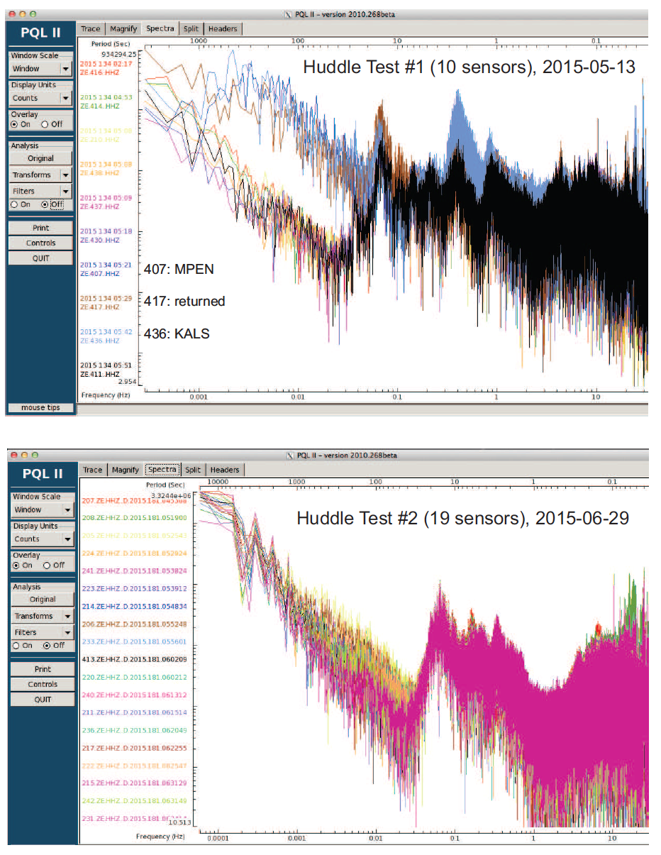
Figure S3. Seismic spectra from two huddle tests for Southern Alaska Lithosphere and Mantle Observation Network (SALMON) project. Both huddle tests were performed overnight at the UAF Marine Science Center in Seward, Alaska. Spectra from the first set of sensors (top) revealed problems with three posthole sensors (407, 417, 436). It appears that these three sensors were damaged in shipping from the PASSCAL Instrument Center in New Mexico to the receiving center in Seward, Alaska. The sensors were shipped in custom-made pelican cases. Spectra from the second set of sensors (bottom) revealed the agreement that one would hope for in such a test. These spectra were not made until the time of servicing, one year after MPEN and KALS had been deployed. See also Figure 11 in the main article.
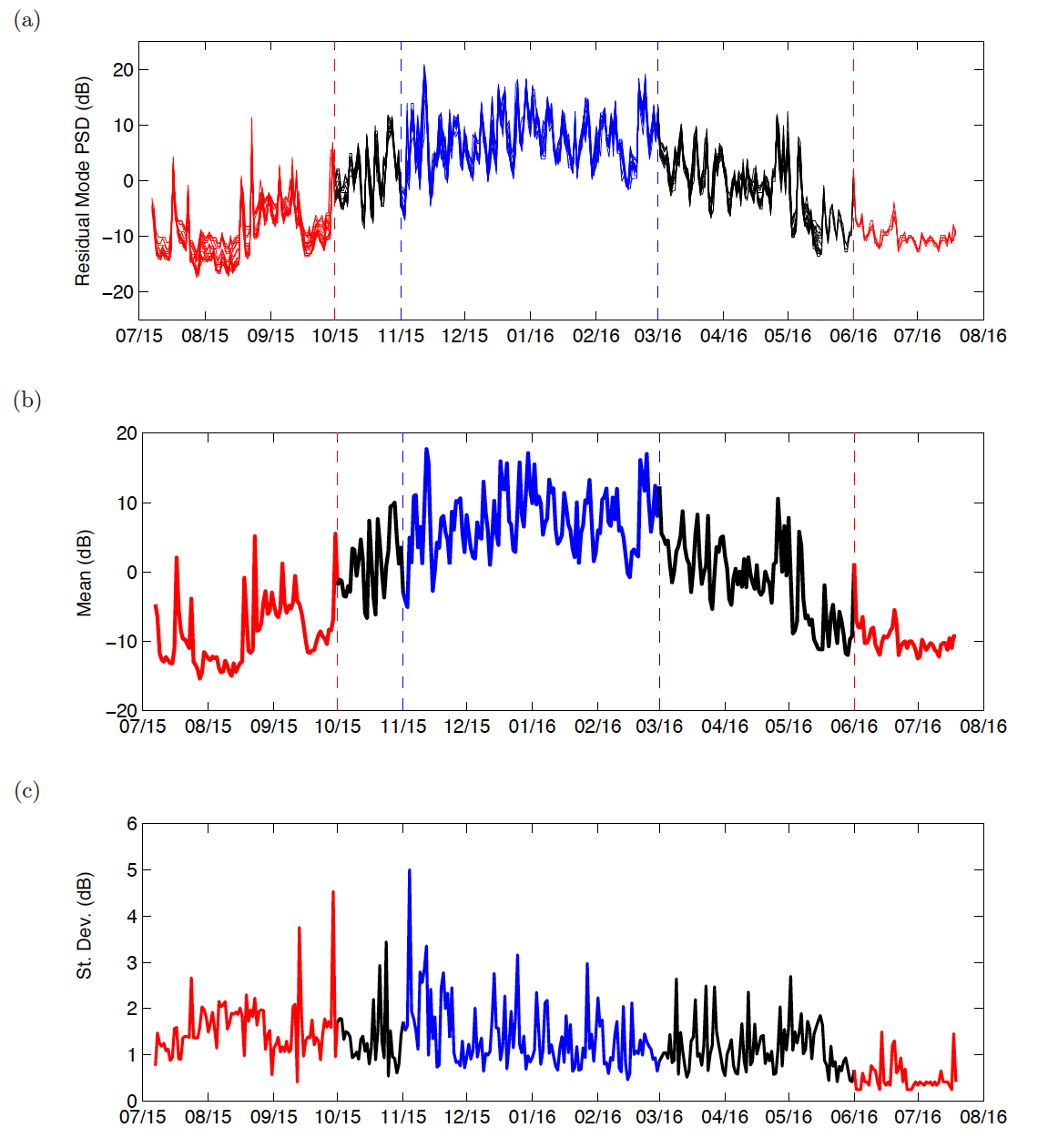
Figure S4. Justification for choosing two different time periods for the analyses of seismic noise. Each time series is colored by time of year: red is summer (from 1 June to 1 October), and blue is the winter (from 1 November to 1 March). The two four-month periods for the seasons are chosen based on the pattern in (a); we use the labels Jun–Sep and Nov–Feb to refer to these. (a) Time dependence of seismic noise at a period of 6 s. For each of the 18 stations, the noise is plotted as the deviation from the annual mean amplitude at 6 s. The extreme correlation among time series shows that all stations in the region experience the same 6-s-period noise fluctuations. Winter exhibits high noise, whereas summer exhibits low noise. Note that for summer 2016 we only have four (out of 18) stations (HLC3, HLC5, WFLS, WFLW), because other stations had already been serviced in May. (b) The mean of the time series in (a). (c) The standard deviation of the time series in (a).
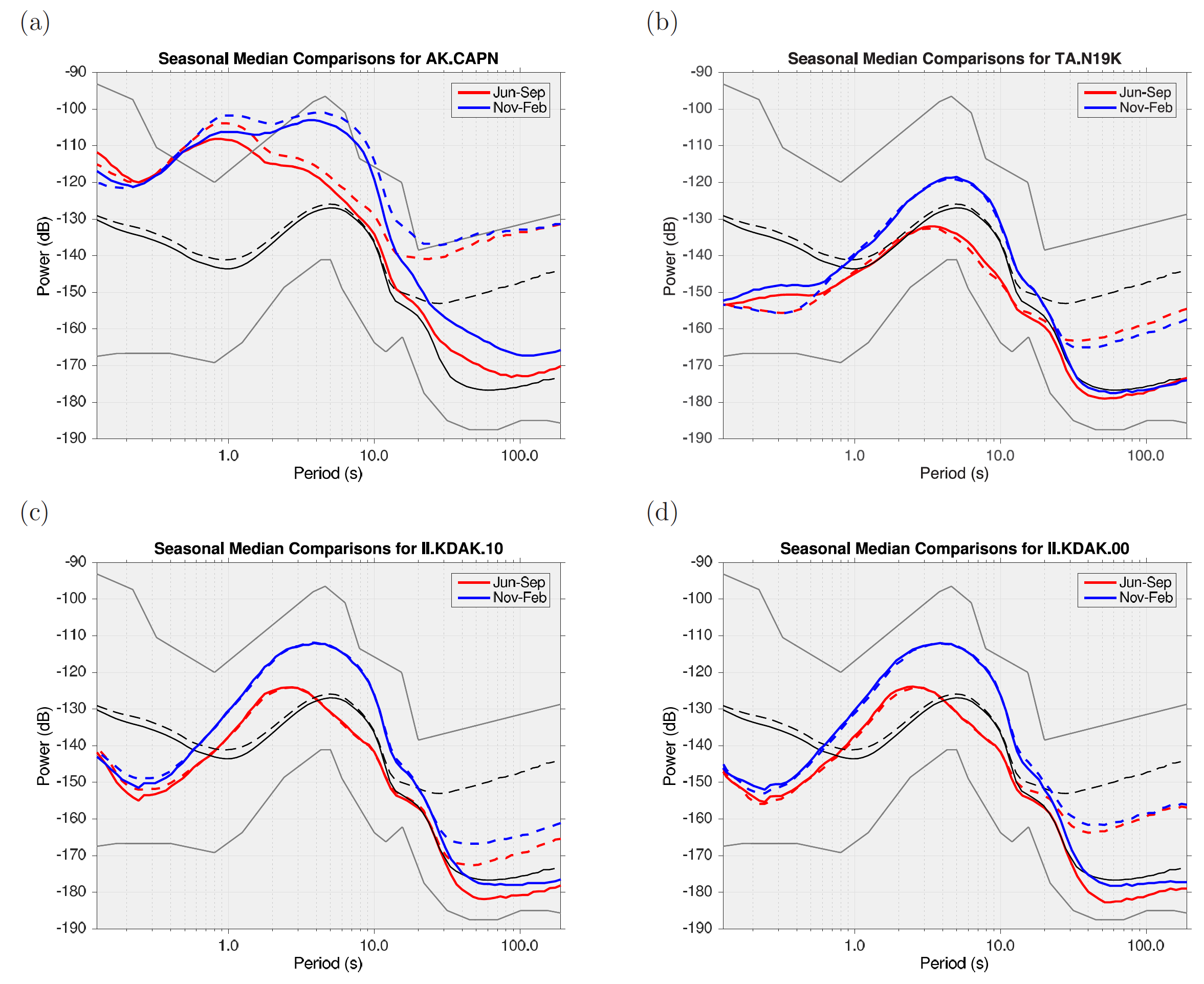
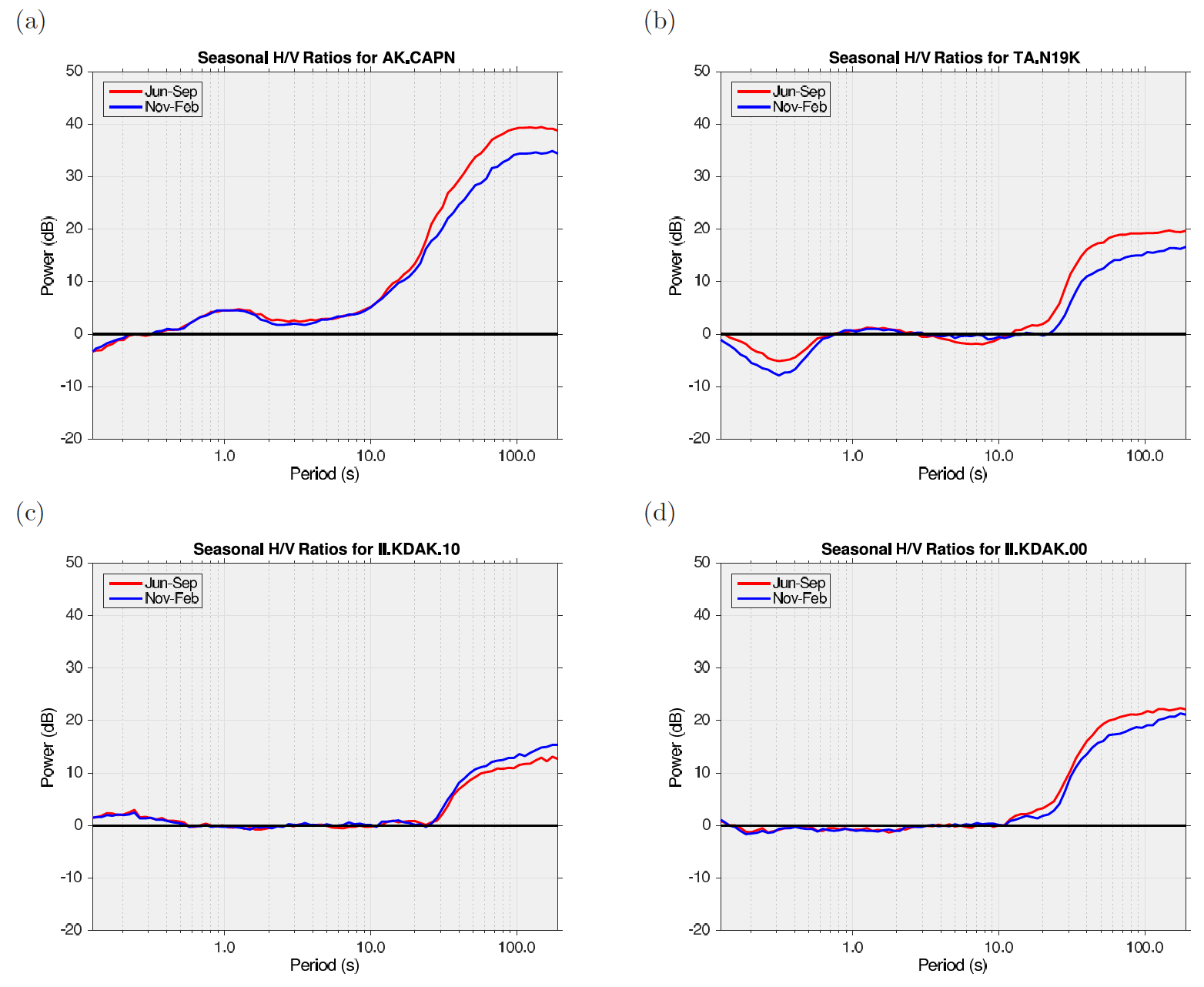
Figure S5. Seismic noise plots for four stations used for comparison with SALMON stations in Figure S6. For each station, the spectra are shown for two different seasons: summer (June–September; red) and winter (November–February; blue). The vertical component is solid, and the mean of the horizontal components is dashed. A stack over all Transportable Array (TA) stations in the lower 48 is shown in black. (a) TA upgrade station AK.CAPN on the Kenai Peninsula. (b) TA station TA.N19K northwest of RV. Overall, TA.N19K is a quieter station relative to the average TA station. (c) Global Seismographic Network (GSN) station II.KDAK.10, a Nanometrics Trillium T120PH sensor in a 5.5-m borehole in bedrock. (d) GSN station II.KDAK.00, a Geotech KS-54000 sensor in an 88-m borehole in bedrock. Over this time period, the shallower sensor exhibits lower horizontal noise levels than the deeper sensor.
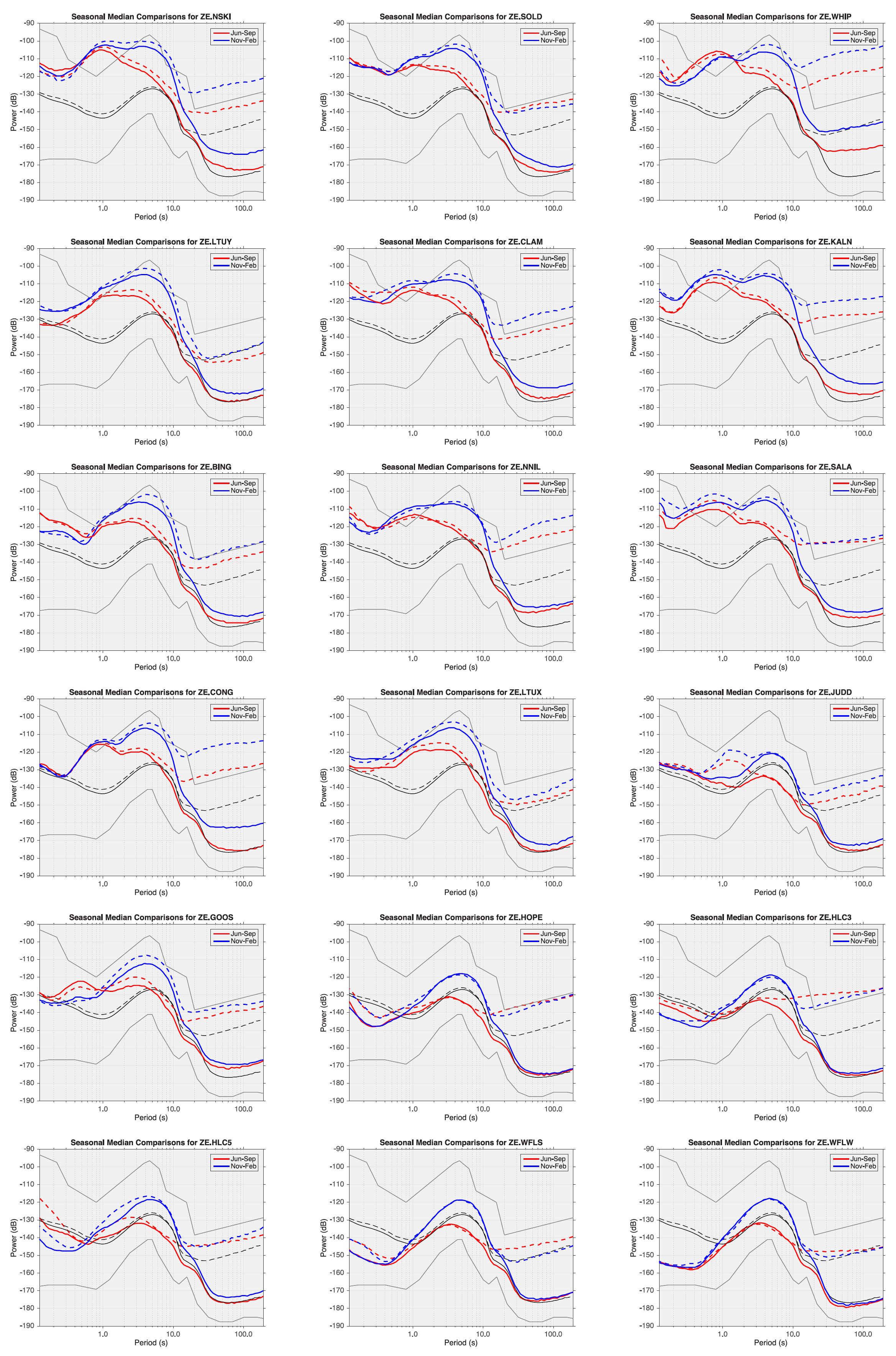
Figure S6. Seismic noise plots for all SALMON stations, ordered by decreasing basin thickness at each station, starting with NSKI (7.0 km) at the upper left and finishing with nonbasin sites (see Table 1 in the main article). Red is summer (June–September); blue is winter (November–February); solid is vertical; and dashed is horizontal. Noise in the winter, especially at periods >2.0 s, is larger than noise in the summer.
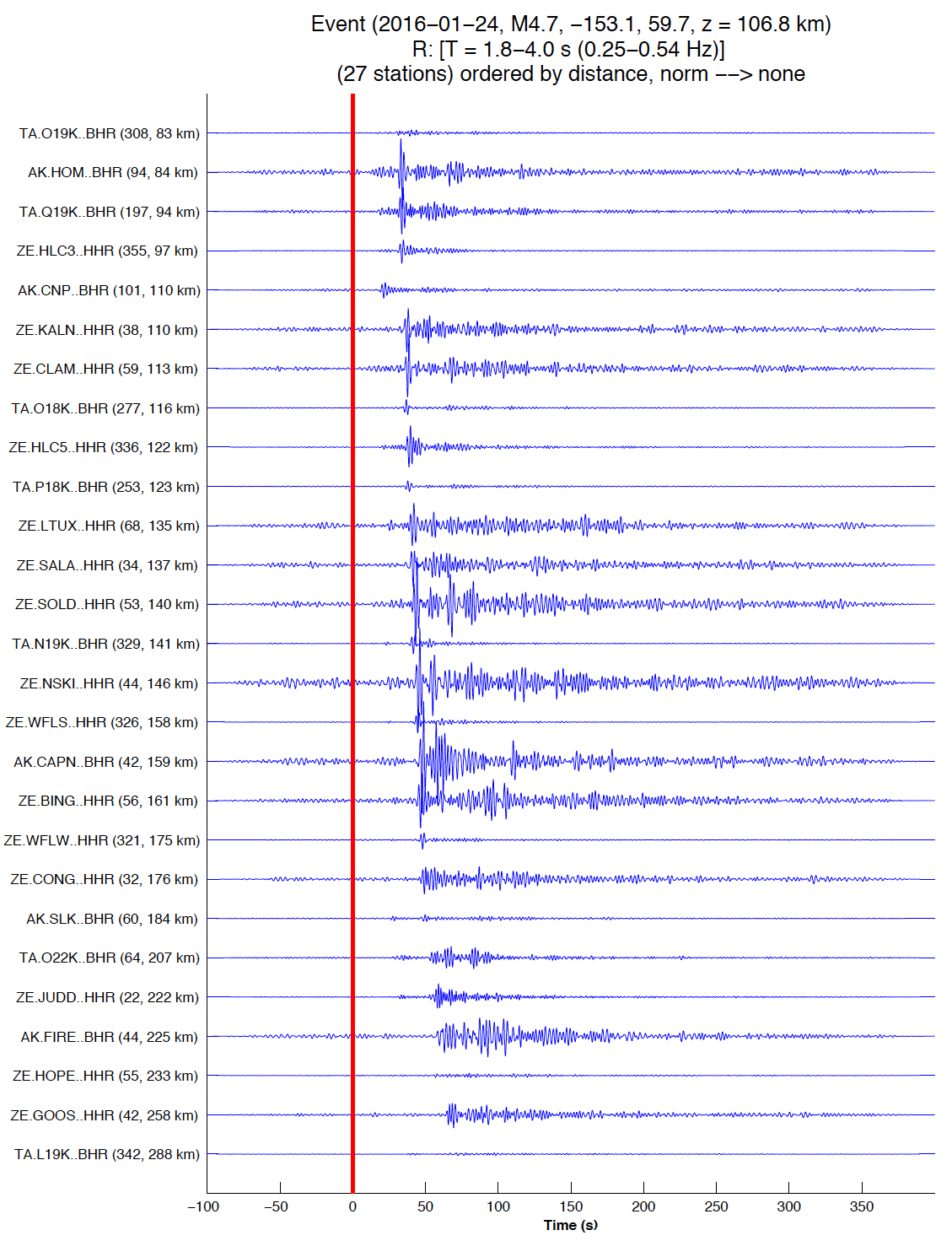
Figure S7. Record section of radial-component seismograms used in the analysis in Figure S11.
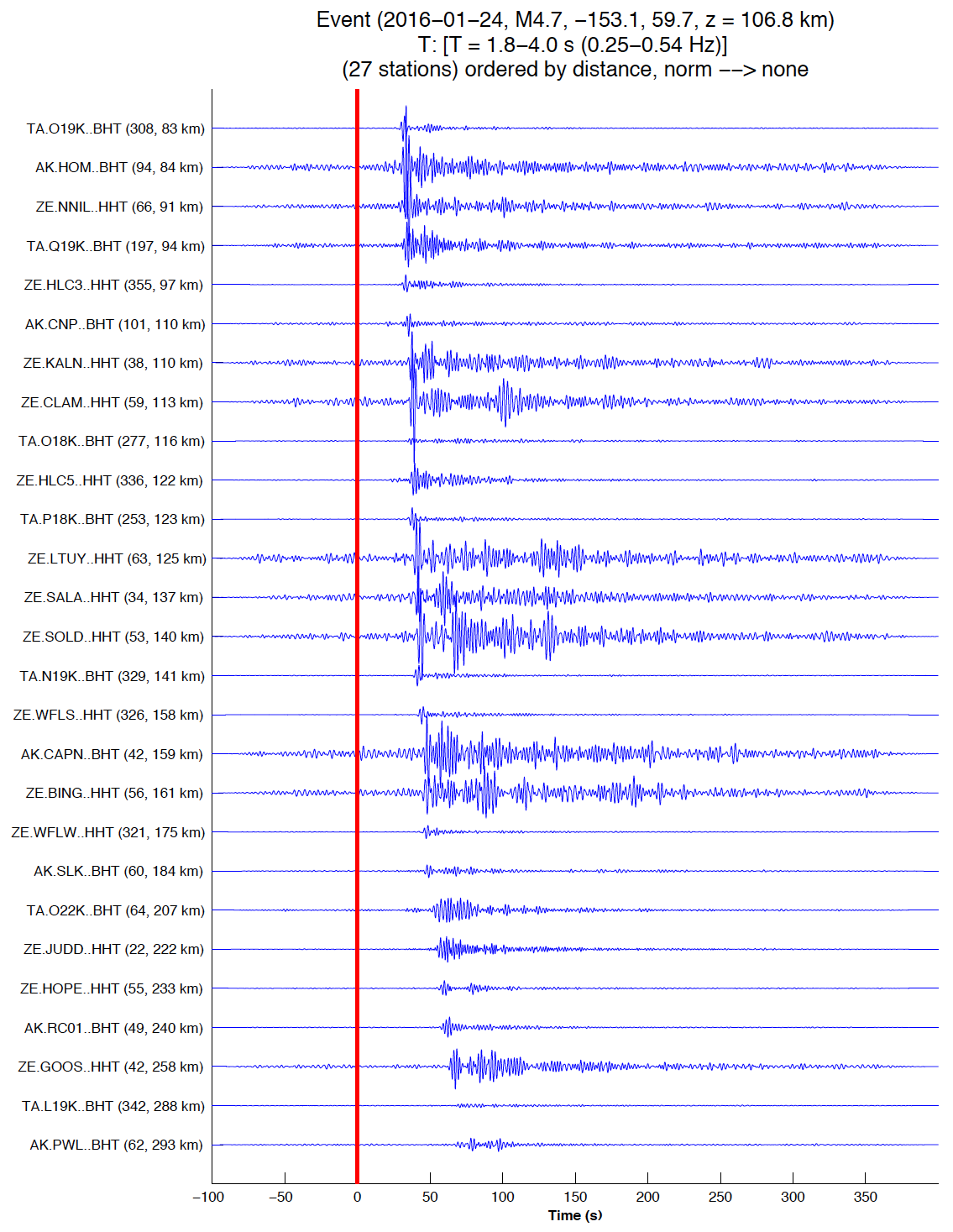
Figure S8. Record section of transverse-component seismograms used in the analysis in Figure S11.
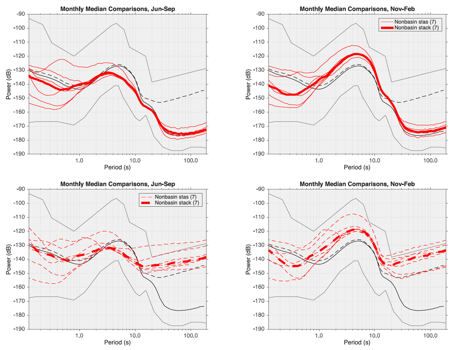
Figure S9. Stacks of spectra for seven nonbasin stations used in our analysis. Left column is summer; right column is winter; top row is for the vertical component; and bottom row is for the mean of the horizontal components. Each stacked spectra was used as a reference in the residual plots in Figures 6c or 7c in the main article.
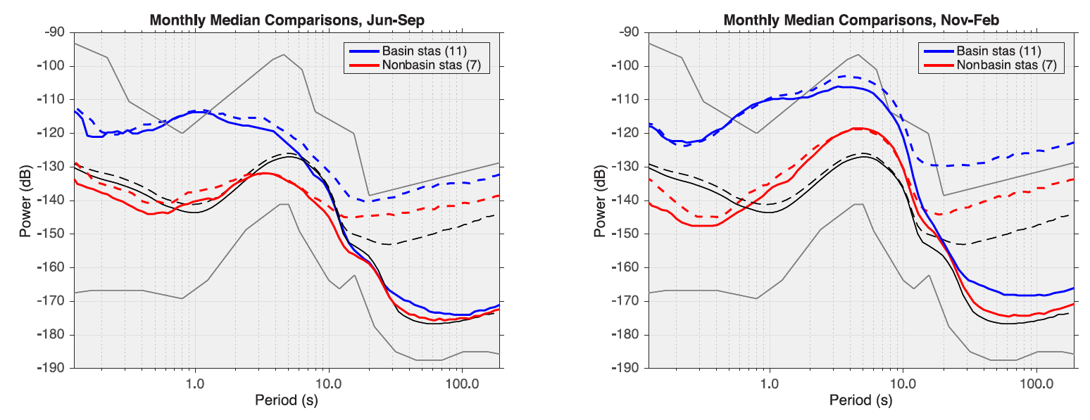
Figure S10. Seismic noise comparison between stacked spectra for 11 basin stations (blue) and seven nonbasin stations (red). See expanded analysis in Figures 6 and 7 in the main article.
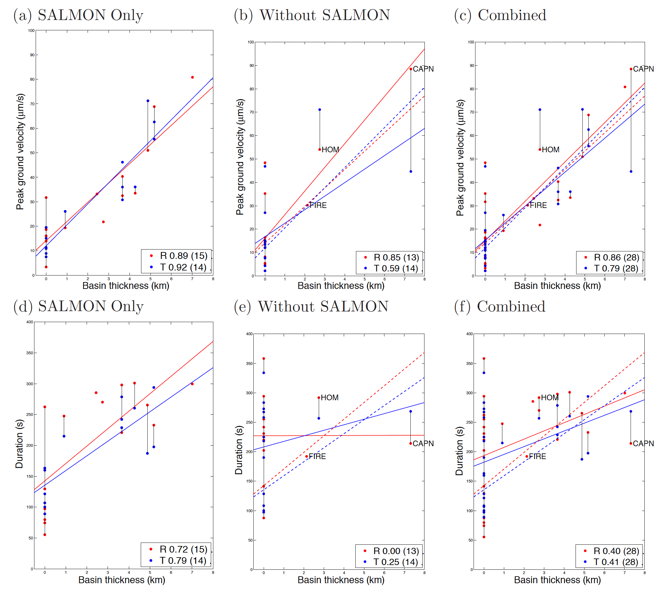
Figure S11. The influence of basin depth (Shellenbaum et al., 2010) on (a–c) peak ground velocity (PGV) and (d–f) duration for an ML 4.7 aftershock (24 January 2016, depth 107 km) of the Mw 7.1 Iniskin earthquake. Seismograms are filtered 1.8–4.0 s and displayed in Figures S7 and S8. Red points and lines denote radial (R) component; blue points and lines denote transverse (T) component. (a) PGV versus basin depth, for SALMON stations only. Seismograms are discarded if they do not meet signal-to-noise ratio criteria. Vertical bars connect the R and T duration estimates for a single station. The legend shows the correlation coefficients of 0.72 (R) and 0.79 (T). (b) Same as (a), but excluding SALMON stations. The dashed lines show the best-fitting lines in (a) for comparison. Non-SALMON basin stations are labeled; these appear in (c) as well. (c) Same as (b) but including all stations in addition to SALMON stations. The correlation coefficients (R 0.40, T 0.45) are lower than those in (a). (d)–(f) Same as (a)–(c), but for duration.
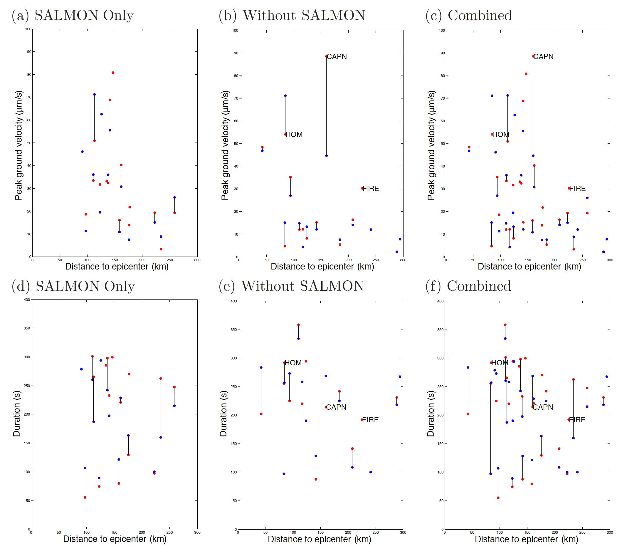
Figure S12. Same as Figure S11, but here the x axis the epicentral distance of each station, instead of basin thickness. Under the approximation of simple, layered Earth structure, we would expect the amplitude of the seismic wavefield to decrease with increasing distance from the epicenter. The overall lack of negative-sloping patterns here implies that the amplitude variations are controlled by nonlayered Earth structure, such as the Cook Inlet sedimentary basin (Fig. S11).
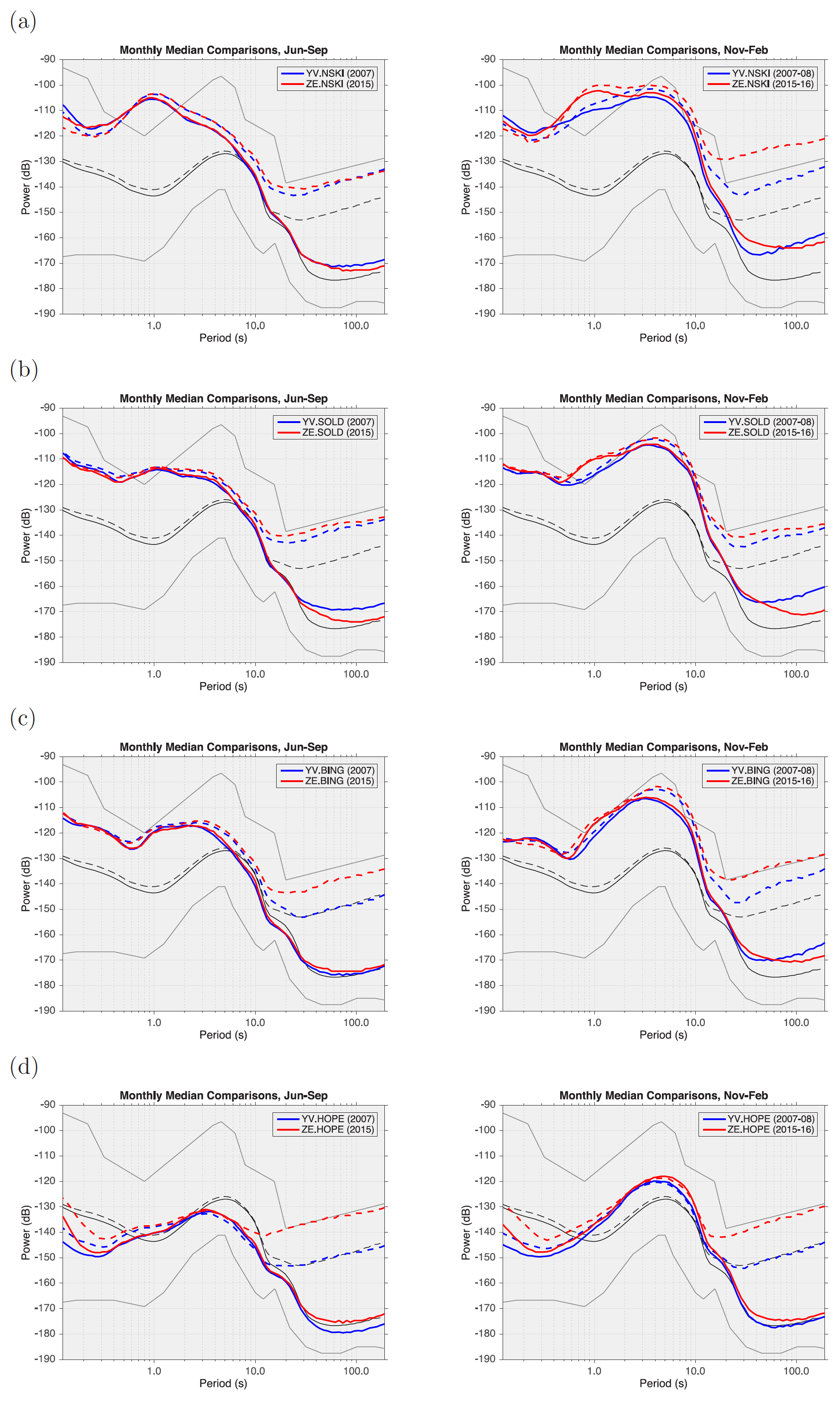
Figure S13. Same as Figure 10 in the main article but for three basin stations (Table 1 in the main article): NSKI (top row), SOLD, and BING. HOPE is a nonbasin station and is repeated from Figure 10 in the main article in the bottom row.
Figure S14. Spectral ratio H/V of the horizontal component to the vertical component for the spectra shown in Figure S5. H/V is largest at long periods, larger for the basin station (AK.CAPN), and larger in the summer.
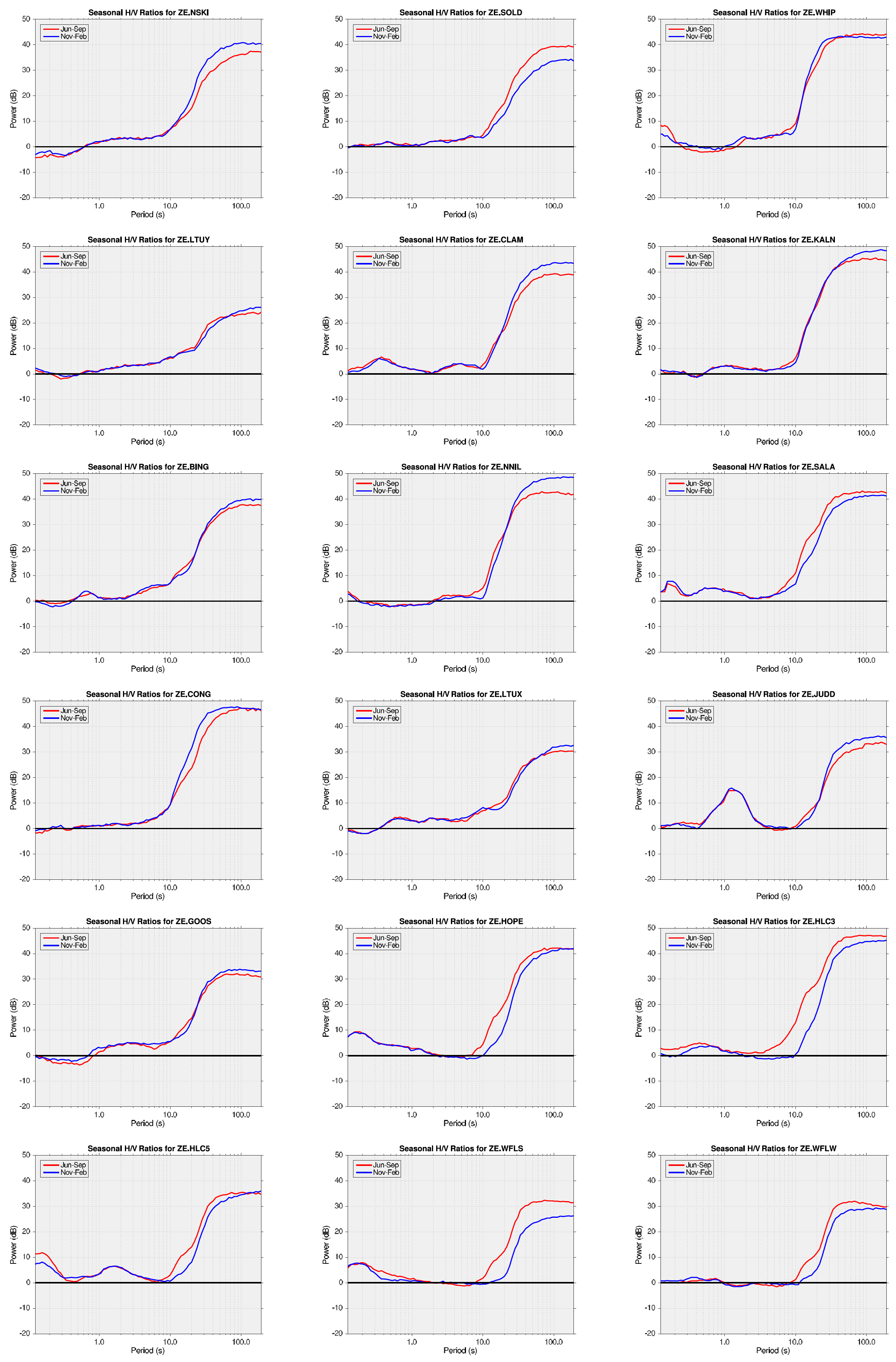
Figure S15. Spectral ratio H/V of the horizontal component to the vertical component for the spectra shown in Figure S6. The plots are ordered by decreasing basin thickness at each station, starting with NSKI (7.0 km) at the upper left and finishing with nonbasin sites (see Table 1 in the main article). Red is summer (June–September); blue is winter (November–February); solid is vertical; and dashed is horizontal.
Eberhart-Phillips, D., D. H. Christensen, T. M. Brocher, R. Hansen, N. A. Ruppert, P. J. Haeussler, and G. A. Abers (2006). Imaging the transition from Aleutian subduction to Yakutat collision in central Alaska, with local earthquakes and active source data, J. Geophys. Res. 111, no. B11303, doi: 10.1029/2005JB004240.
Shellenbaum, D. P., L. S. Gregersen, and P. R. Delaney (2010). Top Mesozoic unconformity depth map of the Cook Inlet basin, Alaska, Alaska Div. Geol. Geophys. Surv. Report of Investigation 2010-2, 1 sheet, scale 1:500,000, available at http://www.dggs.alaska.gov/pubs/id/21961 (last accessed October 2016).
Wang, Y., and C. Tape (2014). Seismic velocity structure and anisotropy of the Alaska subduction zone based on surface wave tomography, J. Geophys. Res. 119, 8845–8865, doi: 10.1002/2014JB011438.
[ Back ]