Figure S1 is a test for scenario 1, in which we compare the snapshots using rise times up to 4 and 10 s. Figure S2–Figure S4 are related to scenario 5. Figure S2 shows the L curves and slip models with increasing smoothness and the selected model. Figure S3 shows fits of the chosen model to the Global Positioning System (GPS) and seismic data. Figure S4 shows the snapshots of the slip rate for scenario 5. Figure S5 shows the high-frequency seismograms of the dynamic simulation at stations near the fault.
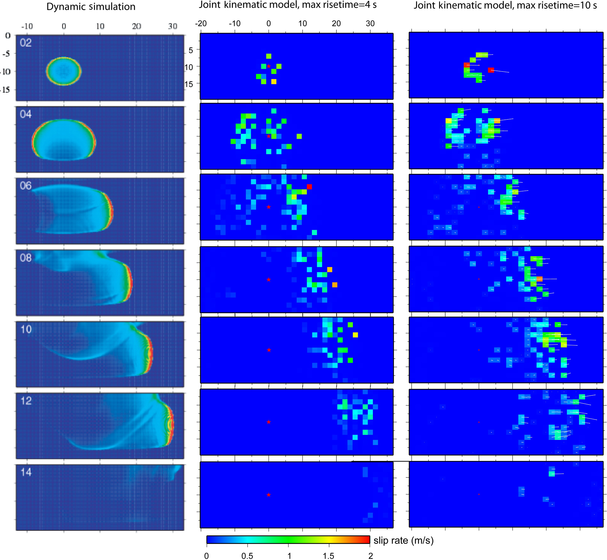
Figure S1. Snapshots of slip rate on the fault every 2 s for scenario 1 for (left) the input model, (center) the joint model with two-parameter rise time with maximum rise time of 4 s, and (right) joint model with two-parameter rise time with maximum rise time of 10 s.
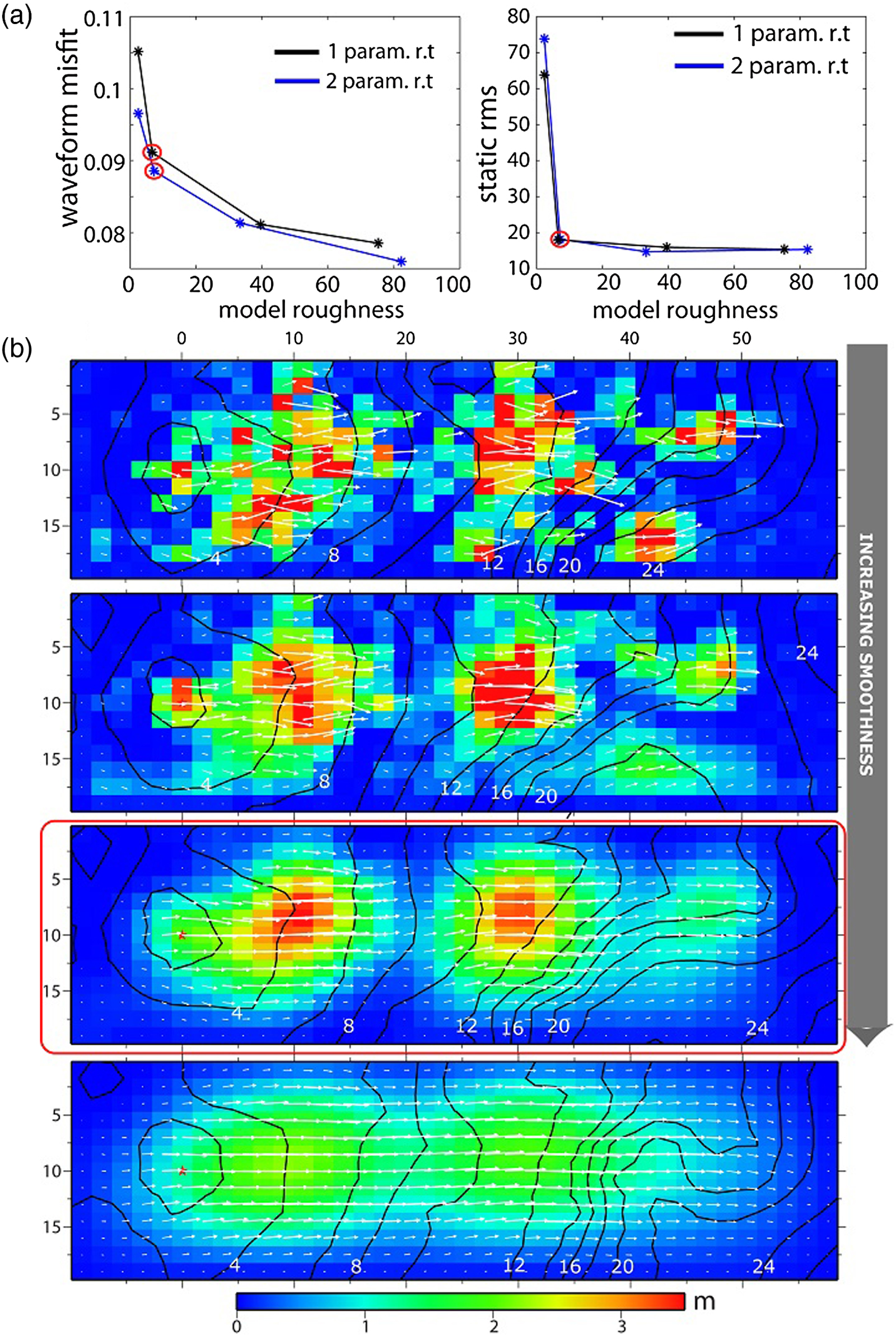
Figure S2. (a) The model roughness versus misfit curves (L curves) for the geodetic and seismic data for scenario 5. The selected best-fit model is shown with a red circle. (b) The slip distributions for the two-parameter rise time (r.t.) joint models with increasing model smoothness from top to bottom. The selected model is shown in a red rectangle.
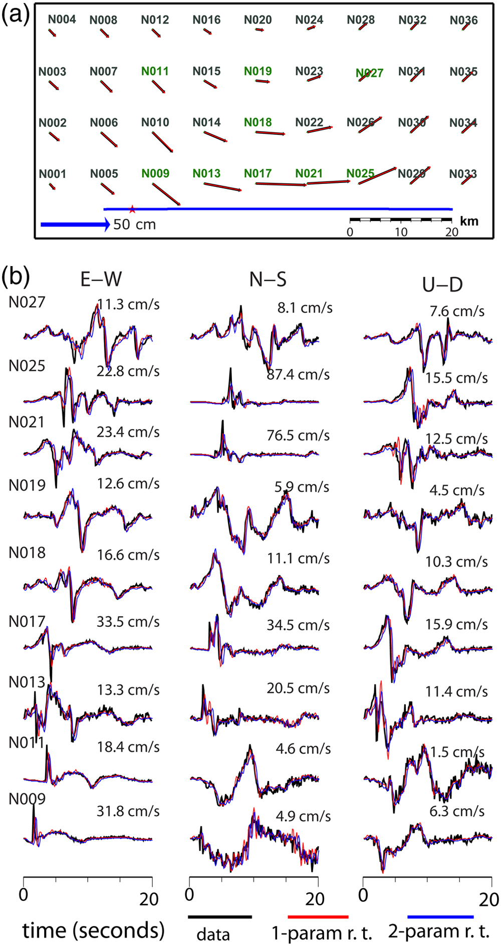
Figure S3. (a) Fits to the geodetic data for the best fit joint model with two-parameter rise time (r.t.) for scenario 5. Data is in black, and fits are in red. The station names are to the top left of the GPS data points. The names of the stations that are also used for seismic data are shown in green. The blue line shows the surface expression of the fault, and the red star represents the epicenter location. (b) Fits to the seismic data at nine stations for one-parameter (red) and two-parameter (blue) rise time joint inversions.
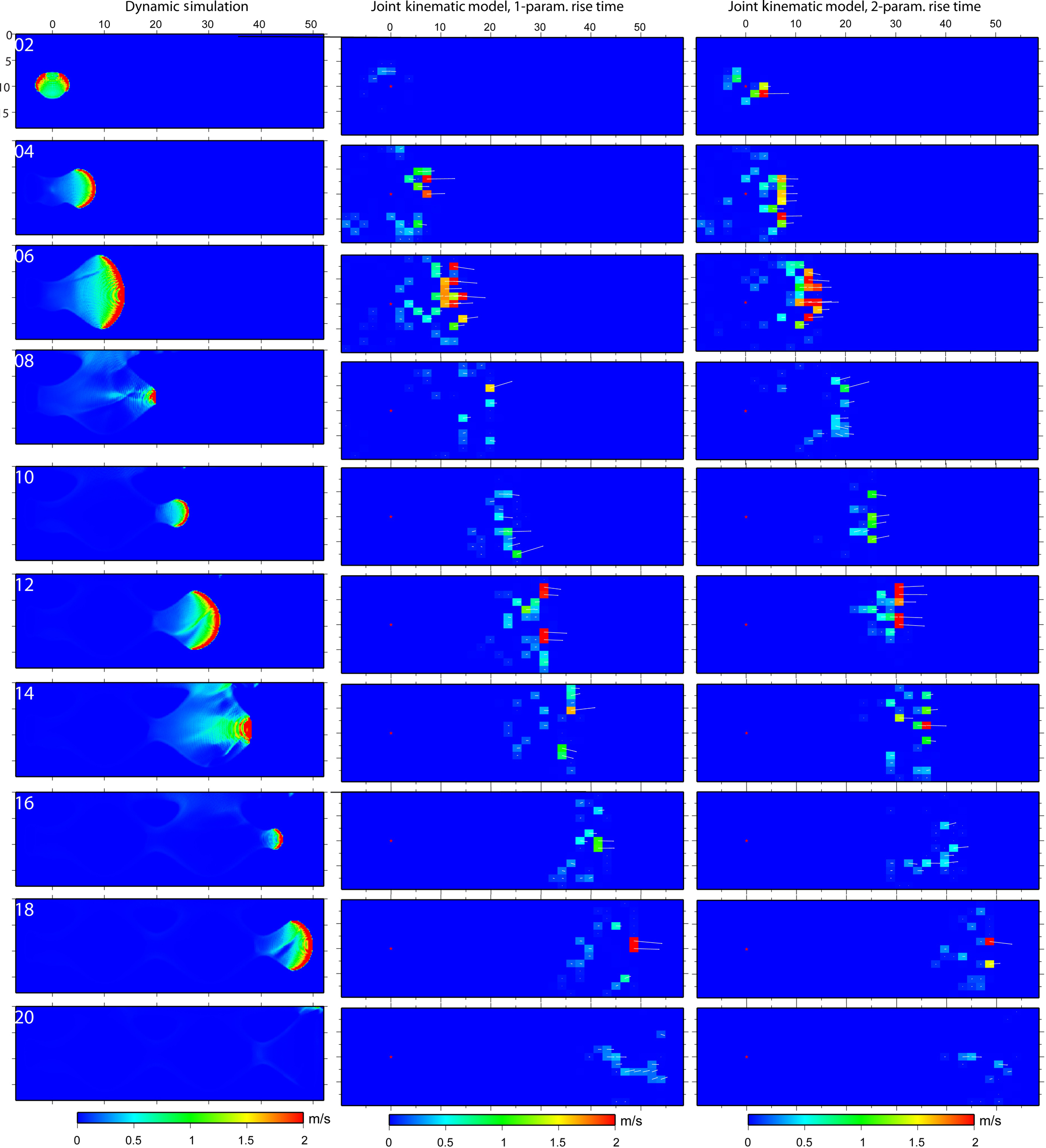
Figure S4. Snapshots of slip rate on the fault every 2 s for scenario 5 for (left) the input model, (center) the joint model with one-parameter slip function, and (right) the joint model with two-parameter slip function. The velocities are saturated at 2 m/s.
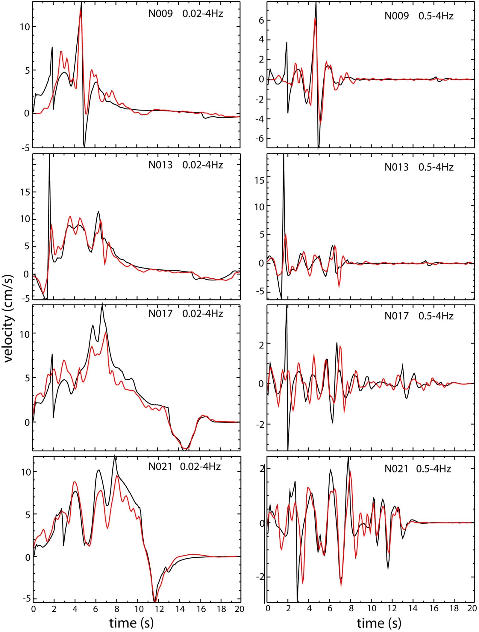
Figure S5. The velocity seismograms at the stations closest to the fault for the scenario 1; the dynamic rupture simulation seismograms are in black, and the fits in red. The left panel shows the broadband (0.02–4 Hz) seismograms, while the right panel shows the high frequency seismograms (0.5–4 Hz).
[ Back ]