This supplement gives a detailed spectral analysis of comb filtering using Butterworth filtering, in conjunction with Ms(VMAX) measurements (Russell, 2006) in order to provide a foundation for a new algorithm to be used for estimating signals below the detection threshold in Rayleigh and Love MsU processing. (MsU is a unified Rayleigh- and Love-wave magnitude scale we designed to maximize available information from single stations and then combine magnitude estimates into network averages.) Specifically, the surface-wave spectrum will be recast as a smoothed spectral estimate from narrowband filtration, followed by analysis of variance, covariance, and correlation due to the narrowband comb filtration. Based on correlation, the effective number of degrees of freedom in the smoothed spectrum will be determined. The analysis will be used to critique the possible use of maximum likelihood censoring for MsU and to propose a more robust censoring method that relies on the strong overlap (high correlation) in the narrowband comb filters across adjacent frequencies. To demonstrate the overall processing used for MsU, the last section gives a pictorial demonstration for the individual steps involved in calculating the MsU event magnitude. In this case, the 2013 Democratic People’s Republic of Korea (DPRK) nuclear explosion is used as an example.
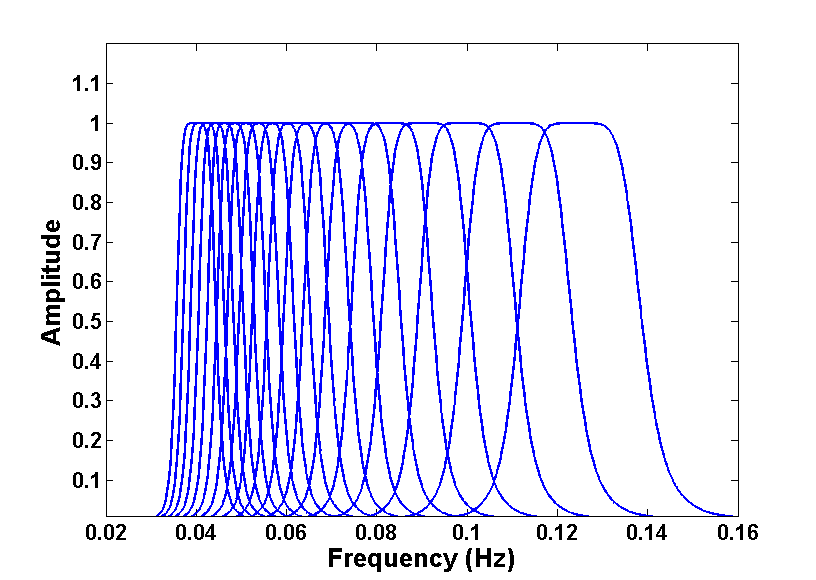
Ms(VMAX) is a method to extend traditional surface-wave magnitude measurements to band ranges with periods broader than 20 s and simultaneously to correct for dispersion errors (Russell, 2006). Traditional surface-wave magnitudes rely on measuring the maximum amplitude of dispersed seismograms, at periods typically between 17–23 s in the time domain. Because strong dispersion spreads the individual frequencies apart in the time domain, the time domain measurements act as a surrogate for frequency domain amplitude measurements. However, this practice can introduce large errors in the presence of Airy phases, where the signals are undispersed. Ms(VMAX) extends the traditional method to frequency bands between 8 and 25 s, narrowband filtering raw seismograms in a comb filter spaced at 1 s intervals and selecting the filter with the maximum amplitude. The filter widths are chosen to minimize dispersion error. Figure S1 illustrates a typical comb filter used for analysis, as a function of frequency. The width of the individual filters changes as a function of the expected dispersion at that frequency, and notice also that the filters are overlapping, which induces correlation across the measurements. These will be discussed in detail below.
The fundamental frequency model used in Ms(VMAX) is based on amplitudes corrected back to the source, as represented in equation (1) in the main paper. Simplifying equation (1) to emphasize the frequency model gives
Acor = A(f,x)S(f )I(f )G(x)Q(f,x),
(S1)
in which Acor is the corrected source amplitude spectrum, A(f,x) is the surface-wave amplitude spectrum measured at frequency f and distance x, I(f ) is the instrument correction, E(f ) is a source excitation correction that is only a function of frequency, F(x) is geometric spreading that is only dependent on the distance x, and Q(f,x) is an attenuation correction that is a function of both frequency and distance. What is important for this analysis is that the basic model is a constant across frequencies, assuming that source and propagation terms in equation (S1) adequately reflect corrections to the spectrum. In practice, the raw spectrum A(f,x) will be narrowband filtered and measured in the time domain, converted to an equivalent spectral measurement, and then the corrections in equation (S1) applied. This is under the assumption that the filters used are narrow enough that the spectrum varies slowly across the width of the filter, and the filtered time domain signal can thus be considered a scaled measure of the spectrum A(f,x).
Russell (2006) gives the basic frequency–time transforms for surface-wave amplitudes at a given frequency (for simplicity, the distance dependence of A(f,x) will be assumed implicitly and the amplitude spectrum written as A(f )):
(S2)
in which
(S3)
In equation (S2), is the maximum filtered time domain amplitude corresponding to the signal group velocity at . The term α, which is a function of frequency, group velocity, and its derivative, represents the dispersion of the seismogram. As α increases, the dispersion increases, and as , the seismogram becomes nondispersive, or an Airy phase. In equations (S2) and (S3), Bn is a zero-phase, nth-order Butterworth filter centered on , and fc is the one-sided width of the filter. Bn has a maximum amplitude of 1 and reduces to 0.5 at . Equation (S3) has been generalized from Russell (2006), in that the origin has been translated back to to emphasize the bandpass filtration, and standard frequencies have been substituted for angular frequencies for convenience.
The essence of the technique in Russell (2006) is to show how equation (S2) can be considerably simplified if the frequency width fc satisfies an inequality dependent on the dispersive term α. Define the Butterworth gain as
(S4)
in which n is the filter order. In the original paper, Russell (2006) demonstrates that if
(S5)
then substituting into equation (S2) will only add a minimum error to the integral; and, if or is slowly varying across the bandwidth of Bn, then a simple solution to equation (S2) can be found:
(S6)
Notice that the integral in (S6) is no longer complex because the complex exponent in equation (S2) is equal to 1 if . Solving equation (S6) for gives
(S7)
As an example, if the order of the Butterworth is n = 3, then Russell (2006, his table 1) shows that the maximum error (ERR) in equation (S7) due to the approximation will be ERR ≤ 0.036 in magnitude units. Also, equation (S5) can be put into the following simplified form from Russell (2006):
(S8)
in which Gmin is a constant, which is a function of the maximum observed dispersion across the 8–25 s frequency band, and Δ is the source–receiver distance in degrees. Notice that from equations (S3) and (S8), the width of the Butterworth filter will change as a function of the frequency , as Figure S1 demonstrates.
Equations (S7) and (S8) form the basis of the Ms(VMAX) technique. These equations show that the maximum amplitude of the filtered time domain signal can be used as a scaled estimate of the spectrum, regardless of the amount of dispersion, under the condition that the filter width obeys the inequality in equation (S8). To construct Ms(VMAX), a Butterworth magnitude formula is constructed by taking the logarithm of equation (S7), incorporating the corrections in equation (S1), and scaling the magnitude to traditional surface-wave magnitudes measured at 20 s. Then, the corrected magnitude can be searched across periods from 8 to 25 s to determine which period gives the maximum magnitude (Bonner et al., 2006). Notice that if equation (S1) is corrected exactly, all magnitudes calculated between 8 and 25 s will have the same value. However, due to additive noise, spectral nulls, variations in attenuation, and three dimensional propagation effects not accounted for in equation (S1), there may be significant variation across the spectrum. Recasting equation (S6) in a stochastic framework can give insight into the effects of the variation and how to estimate equation (S6) in a low signal-to-noise ratio environment. This will be discussed in the next section.
To recast the Ms(VMAX) problem in a stochastic framework, notice first that the terms on the right side of equation (S6) can be rewritten as
(S9)
in which W is now a scaled version of Bn, with an area of 1. Then, equation (S6) can be rewritten as
(S10)
in which is substituted for , indicating that represents a smoothed average of A(f ) across the bandwidth of W, because, by equation (S10), W is an unbiased weighting function of A(f ). If A(f ) is now considered as a stochastic random variable, then is in the standard form of a smoothed spectral estimate (Jenkins and Watts, 1968; Papoulis, 1977). This will allow for statistical modeling of variations in the spectrum due to noise and complexities in the signal not modeled in equation (S1). In the standard theory, the integral limits are usually expressed between −∞, ∞; however, changing to 0, ∞ does not change the statistical analysis, because in this analysis the value of the weighting function W is properly defined over 0, ∞.
To determine the distribution of the amplitude spectrum and then the smoothed distribution of , start by determining the distribution of the power spectrum . For this analysis, errors in the spectrum will be assumed from both signal and noise sources; and, assuming that the signal and noise are considered as statistically independent,
(S11)
Because these are calculated as Fourier transforms of time domain random variables, a suitable distribution for the variables in equation (S11) is a scaled chi-square distribution,
(S12)
The Xk are considered as normally distributed, independent, random variables with mean = 0 and variance = 1, v is the number of degrees of freedom, and c is the scaling constant. Equation (S12) is a very general form for χ2, in that it allows for any mean or variance in the frequency domain, based on varying c and v according to the formulas
mean = μ = cv; and variance = σ2 = 2c2v
(S13)
(Jenkins and Watts, 1968). Normally, the number of degrees of freedom v for spectral estimates at a given frequency is 2, based on transforming time domain periodograms of random noise; however, the more general case is included in this analysis, because large deterministic signals added to noise may have smaller frequency domain variance with increasing magnitude.
The analysis for the amplitude spectrum is similar, but now the distribution is changed because the amplitude is the square root of the signal and noise power:
(S14)
In this case, the random variable A(f ) will be the square root of the chi-square variables, defining a scaled chi distribution as
(S15)
Equation (S15) shows that the number of degrees of freedom for a chi distribution is the same as for chi-squared, and the scaling factor for chi is the square root of the chi-squared distribution. However, it should be emphasized that the mean and variance for a chi distribution is not the square root of the corresponding chi-square mean and variance. The mean and variance of the chi variable can be calculated from the first and second moments of the chi distribution, where Γ is the gamma function:
(S16)
(Forbes et al., 2011). The importance of equation (S16) is that if a random variable is defined as having a chi-squared distribution, the mean and variance of the square root distribution can be found if the scaling factor (c) and number of degrees of freedom (v) are known for the chi-squared distribution.
Because the signal and noise variables in equation (S14) are assumed independent, the means and variances will add:
(S17)
Rearranging equation (S13) in terms of chi-squared degrees of freedom and scaling factor, and substituting in the values into equation (S17), gives
(S18)
Substituting equation (S18) into (S16) gives the mean and variance of the amplitude spectrum in terms of the squared signal and noise spectra:
(S19)
Equation (S19) demonstrates that if the mean and variance of the power spectra of signal and noise are known, then the mean and variance of the amplitude spectrum (S14) can be calculated.
To determine the variance and correlation structure of the smoothed amplitude spectrum in equation (S10), the covariance function (COV) for the smoothed function is
(S20)
(Jenkins and Watts, 1968). Jenkins and Watts include an additional term, W(fk+g); however, it is negligible here due to assuming that the amplitudes of the bandpass filters are negligible at zero frequency, which can be shown to be generally true for standard digital bandpass filter implementation. W is the weighting filter in equation (S10), which has an area of 1, and is the variance of the chi distribution calculated above. Notice also from equations (S3) and (S9) that the width of W at fj will be different than at fk. To scale the covariance properly, tw represents the maximum time domain width used for the sampled Fourier spectrum, or for this analysis, the maximum time domain width used to calculate the narrowband Butterworth filters. Notice that the inverse of tw is equivalent to the sampling width Δf in the frequency domain if discrete Fourier transforms are used. Recall also that the frequency width of W is the same as the Butterworth, 2 fc. This points out a fundamental limitation in using equation (S20), which is that
(S21)
Equation (S21) basically conveys that the one-sided width of the narrowband filter used must be greater than the effective frequency sampling width, or equation (S20) and the following equations below have no meaning.
To calculate the variance of , setting fj = fk in equation (S20) results in (Jenkins and Watts, 1968)
(S22)
From equation (S9) the variance can be written
(S23)
As an example, if the order of the Butterworth filter is 3, the integral in equation (S23) can be calculated as ≈1/(2.5 fc), giving a simple result for the variance of
(S24)
The ratio in equation (S24) is referred to in Jenkins and Watts (1968) as the variance ratio, indicating how much the variance () of the amplitude will be reduced by smoothing.
The correlation between the smoothed spectral estimates is defined as
(S25)
(Jenkins and Watts, 1968), which from equations (S20) and (S22) is defined as
(S26)
Equation (S26) shows that correlation between different frequencies is strictly a function of the overlap of the weighting filters W. Notice also that from equations (S3) and (S9), the width of the weighting filters will be a function of the center frequencies fj and fk, which can be seen from Figure S1.
The importance of the correlation across the spectral band is that it can give a measure of the effective number of degrees of freedom inherent in the total number of measurements. For instance, as was pointed out in the beginning, Ms(VMAX) is usually set up as a narrowband comb filter sampled at 1 s intervals between periods of 8–25 s in the frequency domain. In this case, the total number of possible degrees of freedom is 18; however, due to the strong overlap, the effective number of degrees of freedom may be significantly reduced.
To calculate the effective number of degrees of freedom, equation (S26) can be solved as an autocorrelation sequence (ρ1k, k = 2,3,…n; n = 18) to determine the correlation structure from the lowest to highest frequency (or period). Then, using a formula from Zieba (2010), the effective number of degrees of freedom can be calculated from the correlation structure as
(S27)
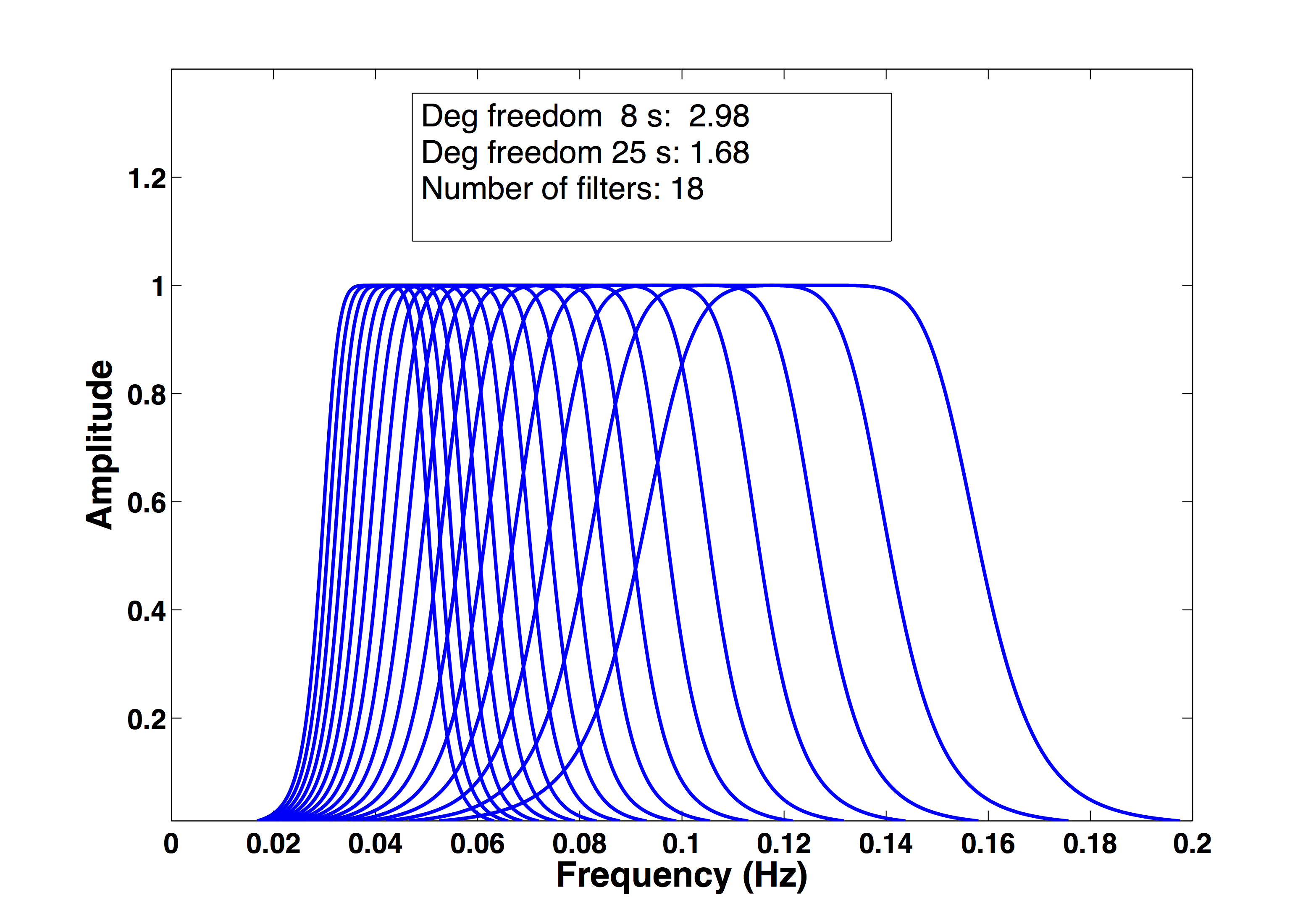
From equation (S27), if the data is completely uncorrelated (ρ1k = 0, k = 2,3,…n), then neff = n. If the data are completely correlated (ρ1k = 1, k = 2,3,…n), then neff = 1. Normally, equation (S27) would give the effective number of degrees of freedom across the measured spectral band. However, because in Ms(VMAX) the overlap changes from low to high frequencies, the correlation structure also changes across the band. Therefore, a range of effective degrees of freedom needs to be calculated: one for the correlation structure at the low end (ρ1k, k = 2,3,…n) and one for the high end (ρnk, k = n-1, n-2,…2). Figure S2 gives an example of this, in which the correlation and range of degrees of freedom are plotted for an event at a 5° source–receiver distance, using equation (S8) with Gmin = 0.6, along with the corresponding comb filter.
It is possible to have a single correlation structure across the spectrum, if the sampling interval is changed from evenly spaced 1 s samples from 8–25 s, to an equivalent logarithmically spaced interval. Letting tmin be the minimum period and tmax the maximum, the logarithmic spacing can be constructed as follows, using MATLAB format:
n = tmax-tmin+1
tloghi = log(tmax)
tloglo = log(tmin)
dlog = (tloghi-tloglo)/(n-1)
tlog = tloglo:dlog:tloghi
Tcnt = exp(tlog)
Tcnt is the vector of logarithmically spaced periods between tmin and tmax. The spacing for 8–25 seconds is shown below in MATLAB format.
Tcnt =
[8.0000 8.5546 9.1476 9.7817 10.4598 11.1850 11.9603 12.7894 13.6760 14.6241 15.6379 16.7220 17.8812 19.1207 20.4462 21.8636 23.3793 25.0000]
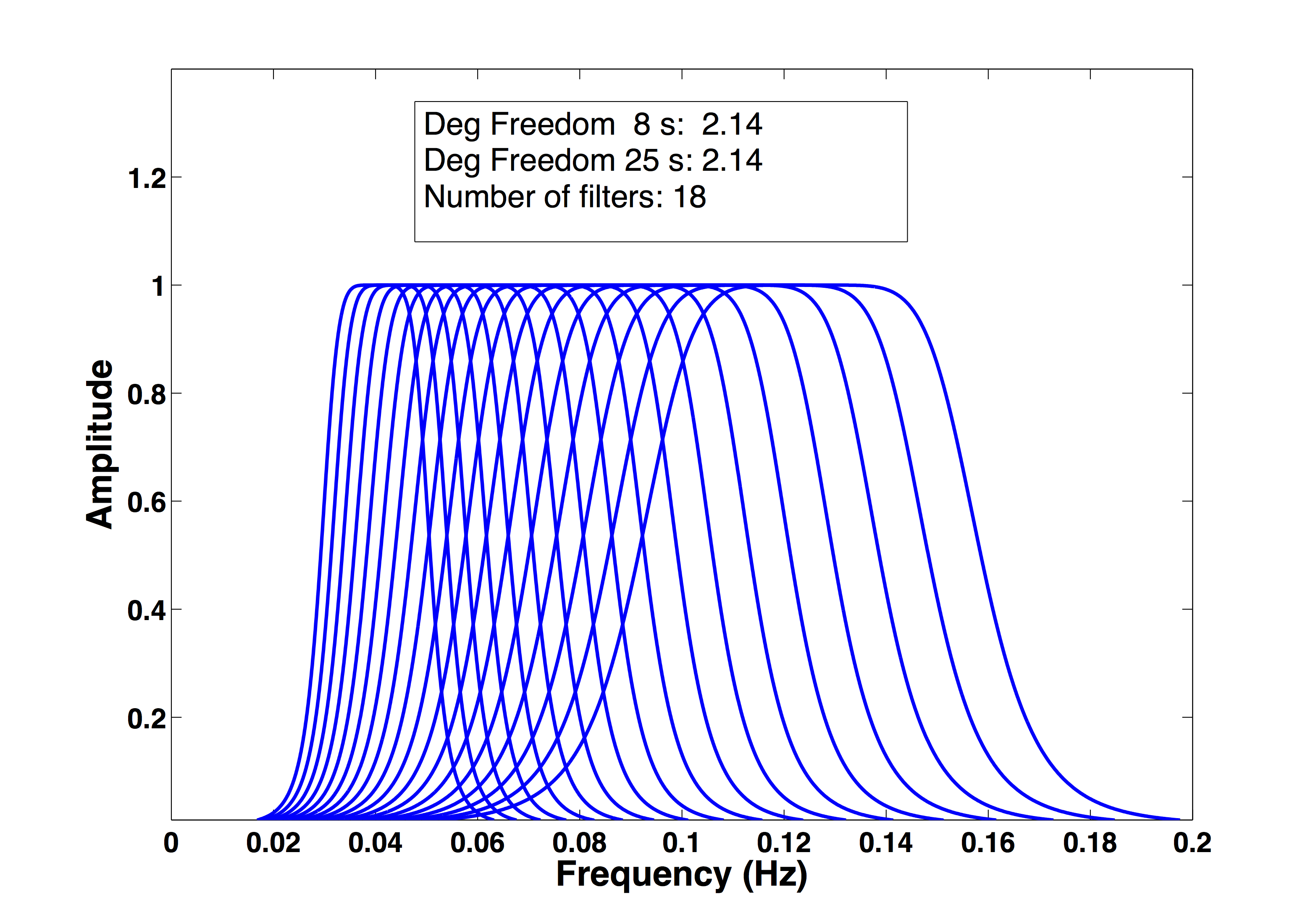
Substituting this spacing into equations (S26) and (S27) shows that logarithmically spaced periods will result in a single correlation structure across the spectrum, with a single effective number of degrees of freedom instead of a range of degrees of freedom. Figure S3 shows that although the widths of the filters change across the spectral band, with logarithmic spacing now the overlap between each adjacent filter remains proportionally constant, resulting in a single correlation structure with an effective number of degrees of freedom of neff = 2.14. This can be shown to be true for any distances, with changing minimum and maximum periods. A proof demonstrating that logarithmic spacing results in proportionally constant overlap between filters is given below. In general, for a third order Butterworth filter with logarithmic period spacing between 8 and 25 s, the effective number of degrees of freedom over the spectral band will vary with source–receiver distance from neff = 1.5 at 2° to neff = 6 at 50°, using a value of Gmin = 0.6. Notice that changing the number of sampling points to a larger number does not increase the effective number of degrees of freedom, because the overlap also increases. For example, if in the above case the maximum number of comb filters between 8 and 25 s is changed from 18 to 50, the calculated effective number of degrees of freedom changes from 2.14 to neff = 2.08. This again shows that the effective number of degrees of freedom is proportional to the filter overlap, and not the number of filters used. It is recommended that logarithmic spacing be used for Ms(VMAX) processing, because it will result in proportionally constant overlap across the spectral band, with a single effective number of degrees of freedom representing the spectral correlation structure.
This section offers a short proof for the conjecture that logarithmic period spacing results in uniform overlap of Butterworth comb filters. Define any two adjacent periods between a minimum tmin and maximum tmax as T1 and T2. Also let the one-sided filter widths of the Butterworth be defined at a given distance x as in Ms(VMAX):
(S28)
in which C is a constant.
Define the uniform logarithmic spacing interval as
ΔT = [log(tmax–log(tmin)]/(n−1),
(S29)
in which n is the number of points. Therefore, for any two adjacent periods,
ΔT = log(T2–log(T1 = log(T2/T1).
(S30)
Take the antilog of equation (S30) for
T2/T1 = exp(δT) = D,
(S31)
in which D is a constant. Equation (S31) can be interpreted as saying that for logarithmic spacing, any two adjacent periods are directly proportional to each other. Note that because frequency is the inverse of period, f = 1/T, and equation (S31) can be rewritten as
f1/f2 = exp(ΔT) = D
(S32)
or
f1 = Df2.
(S33)
The spacing between adjacent frequencies can therefore be defined as
W12 = f1−f2 = Df2−f2 = (D−1)f2 = Ef2,
(S34)
in which E is a constant equal to (D−1). Equation (S34) states that for logarithmic spacing, the width between adjacent frequencies is directly proportional to the lower frequency . Writing the filter width in equation (S29) in terms of frequencies gives
fc2 = C/T2 = C/f2.
(S35)
Substituting equation (S35) into (S34) gives the final result
(S36)
in which G is a constant equal to E/C. Rewriting equation (S32) as
f2/f1 = 1/D
(S37)
and then repeating the steps in equations (S33) through (S36) results in
∴ W12 = Hfc1,
(S38)
in which H is a constant.
Equations (S36) and (S38) complete the proof, stating that for logarithmic spacing, the width W12 between any two adjacent frequency points and is directly proportional to the corresponding filter widths and . Therefore, the overlap between any two adjacent filter widths will be constant, and therefore uniform across all frequencies defined between fmin and fmax.
Although MsU will reduce the requirement for large station sampling and azimuthal coverage, it now introduces the censoring problem at the station measurement level, instead of the traditional network averaged level. This is due to the observation that in many cases, especially at lower magnitudes, either the Rayleigh or Love phase measured at a station will be below the signal detection threshold at some or all periods between 8 and 25 s. It is essential that a censoring method be utilized to estimate signals in noise across the frequency band so that MsU can be routinely calculated for smaller events without introducing significant bias in the averaging process due to nondetecting phases. There are a number of approaches to censoring that are commonly used in seismic network analysis, the most popular being maximum likelihood estimation (MLE), based on standard statistical likelihood analysis of sampled data with assumed probability distributions. This will be reviewed in depth for possible use in the MsU problem, and other alternatives will be proposed, based primarily on the smoothed correlation analysis presented in the sections above.
In network seismology, the traditional approach to left censoring, defined as analyzing magnitudes below detection thresholds as a part of network averaging, relies primarily on assumed statistical data distributions and using a likelihood function to determine means and variances of overall network magnitudes. The likelihood function is defined in terms of conditional probabilities on the mean and standard deviation as follows.
(S39)
P(…|…) = conditional probability
μ = event mean value
σ = event standard deviation
M = station magnitude corresponding to the statistical model Mi = μ+vi, in which vi is a random variable with zero mean
= number of detecting stations
= number of non-detecting stations
m = vector of observed station magnitudes (dimension n1)
d = vector of observed station detection thresholds (dimension n2)
The event mean and standard deviation μ, σ can be estimated from the values that maximize the likelihood function L in equation (S39). If all stations are detecting ( ), it can be shown that equation (S39) reduces to a simple network sampling average for μ and σ, under the assumption of a normal probability distribution (Jih and Baumstark, 1994). To minimize station bias, it is also assumed that observed station magnitudes have been corrected for distance-dependent propagation effects such as geometrical spreading and attenuation.
This MLE has been successfully used for seismic network censoring by multiple authors, starting with Ringdal (1976). Jih and Baumstark (1994) extended the method to both left and right censoring (clipping) and showed how the solution to equation (S39) in terms of μ, σ can be found through a straightforward iterative technique, assuming normal distributions. However, a drawback of the MLE method for seismic event magnitude estimation is the requirement that a reasonably large number of observations need to be made, with broad azimuthal coverage, because earthquakes will produce radiation patterns that can result in severely biased magnitude estimates if the sampling or azimuthal coverage is small. Also, the fundamental assumptions inherent in effectively utilizing the MLE estimator in equation (S39) for censoring are no longer valid in the single-station phase averaging problem for MsU using Rayleigh and Love amplitudes. MLE assumes that the underlying statistical distribution for censored and measured phases is the same in terms of the mean and standard deviation, but the Love and Rayleigh station phases will inherently have different statistical distributions, in μ (mean) and in σ (standard deviation), due to propagation and radiation pattern differences. What this does to an MLE formulation is to decouple the averaging problem in equation (S39) to separate MLE estimates for Love and Rayleigh waves. In this case, for single stations the only option is to utilize the available data set of measurements across the spectral band, assuming there are enough data degrees of freedom to make MLE viable:
(S40)
(S41)
The subscripts i,j are now assumed across periods between 8 and 25 s instead of for separate stations. The MLE estimates for μR, μL can then be substituted as mean estimates for the Rayleigh and Love amplitudes and the values averaged in equation (S40) and (S41). A chi distribution is assumed for P(…) on the Rayleigh and Love amplitudes, but with differing means and standard deviations. However, applying this form of MLE across the spectral band will result in significant issues and limitations:
Due to the above issues—low degrees of freedom for viable MLE and lack of flexibility in determining maximum values across the spectral band—alternatives to applying MLE to phase censoring for MsU may be more appropriate. A more robust method suitable to fewer degrees of freedom and correlated data is possible, taking advantage of all available information across the spectral passband between 8 and 25 seconds. This information will be integrated in a staged approach to MsU estimation, as outlined below.
The fundamental approach to MsU censoring is to make estimates of signal-in-noise amplitudes for Love and Rayleigh phases separately, at each period between 8 and 25 seconds, based on signal and noise characteristics across the spectral band. These characteristics are based on two assumptions: (a) because the smoothed spectral estimates are highly correlated across the spectral band, there will be continuity of signal across the signal–noise transition points as a function of period; and (b) because the measured data in the signal window have been corrected for propagation and source effects as a function of period, a suitable model estimate for the signal across the spectral band is a constant. Using these assumptions, the following calculations and corrections will be made for each phase separately, in order to estimate signal-in-noise amplitudes for each phase:
After correcting each phase for censoring in steps 1–6, the data for Love and Rayleigh phases will be averaged and MsU calculated as a maximum magnitude across the spectral band. However, two additional checks on the censored data will be made to ensure viable phase averaging:
Formally, the algorithm can be described in a simple mathematical algorithm, using the following variable conventions, where n is the total number of periods used. Let equal an estimate of a bound on the narrowband-filtered noise level at the ith period; for instance, 95% upper confidence bounds on noise can be used or, more empirically, the largest narrowband-filtered noise value in a noise window prior to the signal can be used as an estimate. This assumes that the noise mean and variance are stationary through the signal window, and the bound on noise can be used as an upper estimate of noise strength.
SNR = an empirically determined signal-to-noise ratio multiple of the noise threshold, defining a signal threshold
Zi = SNR × is the signal threshold at the ith period
= narrowband-filtered data measured in the signal window at the ith period
= narrowband signal estimate at the ith period
For j=i+1, …, n, if and , then
(S42)
(S43)
The algorithm also works in reverse, for i-j, j = i-1, …, 1. For multiple thresholds, in which the amplitude is going below the threshold at period i and then going above at period k, the upper bound , i<j<k will be considered as the signal estimate. For amplitudes that are completely below the threshold for all periods, then the minimum amplitude measured across all periods is used as a substitution estimate for the signal , i=1, …, n.
Basically the algorithm states that if an amplitude falls below the signal threshold, then it is considered an upper bound on the signal. In case 1 (S42), if it stays below the threshold value at i, then due to the continuity of highly correlated overlapping filter bands, a reasonable estimate for the signal is the upper bound. However, in case 2 (S43) if the amplitude starts increasing in value due to additive noise, the upper bound as an estimate should be replaced by the threshold Zi, under the assumption that the estimate should follow the constant corrected signal model in equation (S1). Essentially, the signal estimate is either estimated by the upper bound or is corrected for additive noise down to the constant signal model.
The censored estimate is intended for use as an auxiliary phase to constrain averages for independent simultaneous station measurements when combining Love and Rayleigh phases. It is not recommended for use as a stand-alone phase measurement; and, when using both Love and Rayleigh, at least one phase should have an amplitude above the signal detection threshold at a given period.
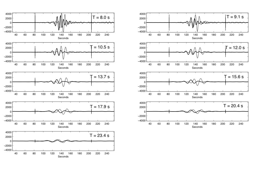
The following describes a step-by-step process of calculating MsU for an event at a single station. The example event is the 2013 DPRK nuclear test at station MDJ, a distance of 370 km from the DPRK test site. The first step in the MsU processing is narrowband filtering the amplitudes, as discussed in the Ms(VMAX) Spectral Analysis section; this involves narrowband filtering the vertical (Z) and transverse (T) components, which represent the Rayleigh and Love amplitudes respectively, between 8 and 25 s (Fig. S4). The next step, as described in the MsU Censoring section, is to apply the censoring method to ensure a stable estimate for both Love and Rayleigh signals across the period band of interest, even when the measured data drops below the signal-to-noise ratio threshold. In this example, the measured data always remain higher than the threshold, and therefore the censored estimate is identical to the measured data (Fig. S5). Next, MsU is calculated at each period using equation 3 in the main article. The period where MsU is calculated to be the highest value is chosen as the MsU value for that station; in this example with station MDJ, the max MsU = 3.79 and is at a period of 8 s (Fig. S6). Then, this whole process would be run for each station that recorded a particular event; in this example, there were seven stations that recorded the 12 February 2013 DPRK explosion included in the processing (Fig. S7). Finally, a network average is calculated with the max MsU value from each station, and that average is the final MsU value for an event.
Figure S1. Ms(VMAX) comb filter between 0.04 and 0.125 Hz at 30° source–receiver distance.
Figure S2. Comb filter plotted for 5° source–receiver distance. Degrees of freedom are calculated at 8 s (0.125 Hz) and 25 s (0.04 Hz).
Figure S3. Same as Figure S2, but with logarithmic spaced periods showing even overlap between filters. Degrees of freedom are now the same at all frequency points (2.14).
Figure S4. Narrowband-filtered waveforms of Rayleigh (gray) and Love (black) waves between 8 and 25 s. The largest amplitudes for both Rayleigh and Love waves are visibly at 8–9 s.
Figure S5. Corrected amplitudes for Rayleigh (gray) and Love (black) waves versus period. The solid lines are the measured data from the vertical (Z; gray) and transverse (T; black) components. The crosses are the censored data points for Rayleigh waves and the circles are the censored data points for the Love waves. The dotted lines represent the signal-to-noise ratio detection thresholds for Rayleigh and Love waves. The censored estimates match the measured data at all periods because all amplitudes were above their respective signal-to-noise ratio thresholds. Also, there is now a smoothed spectral estimate across all the periods due to narrowband filtration.
Figure S6. MsU is calculated from equation 3 in the main article at every period based on the corrected amplitudes shown in Figure S5. At 8 s (black dot), MsU is the highest value; therefore, that value, 3.79, is the picked MsU value for station MDJ from the nuclear test on 12 February 2013.
Figure S7. MsU was calculated at seven stations for the nuclear test on 12 February 2013. At each of these stations, the surface-wave amplitudes were narrowband filtered, and the period with the highest calculated MsU value was chosen to be the MsU value for each particular station. The circles represent the average MsU magnitude calculated for the event, which changes over time as each station updates the event magnitude as the surface waves are recorded. The error bars are the standard deviations around the network average. These MsU values are plotted with respect to approximate time after the origin. The first data point around 2 min is solely from station MDJ, the station of interest in this example.
Bonner, J. L., D. Russell, D. Harkrider, D. Reiter, and R. Herrmann (2006). Development of a time-domain, variable-period surface wave magnitude measurement procedure for application at regional and teleseismic distances, Part II: Application and Ms–mb performance. Bull. Seismol. Soc. Am. 96, 678–696.
Forbes, C., M. Evans, N. Hastings, and B. Peacock (2011). Statistical Distributions, Fourth Ed., John Wiley and Sons, Hoboken, New Jersey.
Jenkins, G. M., and D. G. Watts (1968). Spectral Analysis and its Applications, Holden-Day, Oakland, California.
Jih, R.-S., and R. R. Baumstark (1994). Maximum-likelihood network magnitude estimates of low-yield underground nuclear explosions, TBE-4617-3, Teledyne-Brown Engineering, Arlington, Virginia.
Papoulis, A. (1977). Signal Analysis, McGraw-Hill, New York, New York.
Ringdal, F. (1976). Maximum likelihood estimation of seismic magnitude, Bull. Seismol. Soc. Am. 66, 789–802.
Russell, D. R. (2006). Development of a time-domain, variable-period surface wave magnitude measurement procedure for application at regional and teleseismic distances. Part I—Theory. Bull. Seismol. Soc. Am. 96, 665–677.
Zieba, A. (2010). Effective number of observations and unbiased estimators of variance for autocorrelated data—An overview. Metrol. Meas. Syst. 17, no. 1, 3–16.
[ Back ]