Electronic Supplement to
Transtensional Tectonics of the Minto Flats Fault Zone and Nenana Basin, Central Alaska

Carl Tape, Vipul Silwal, Chen Ji, Laura Keyson, Michael E. West, and Natalia Ruppert

Overview

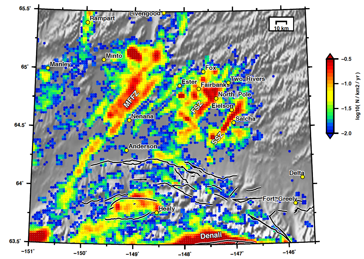
Figure S1 shows the northeast-striking seismic zones in the Fairbanks region of central Alaska (e.g., Page et al., 1995). The focus of this study is on the Minto Flats fault zone (MFFZ). This supplement contains waveform fits (Fig. S2) and depth results (Fig. S3) for the moment tensors listed in Table 1 in the main article. Figures S4 and S5 show variations in seismicity among the subregions of the MFFZ. Figures S8–S13 show how we identified the likely fault plane for the 1995 M_w 6.0 Minto earthquake (Fig. 11 in the main article).

Waveform Fits for Moment Tensor Inversions

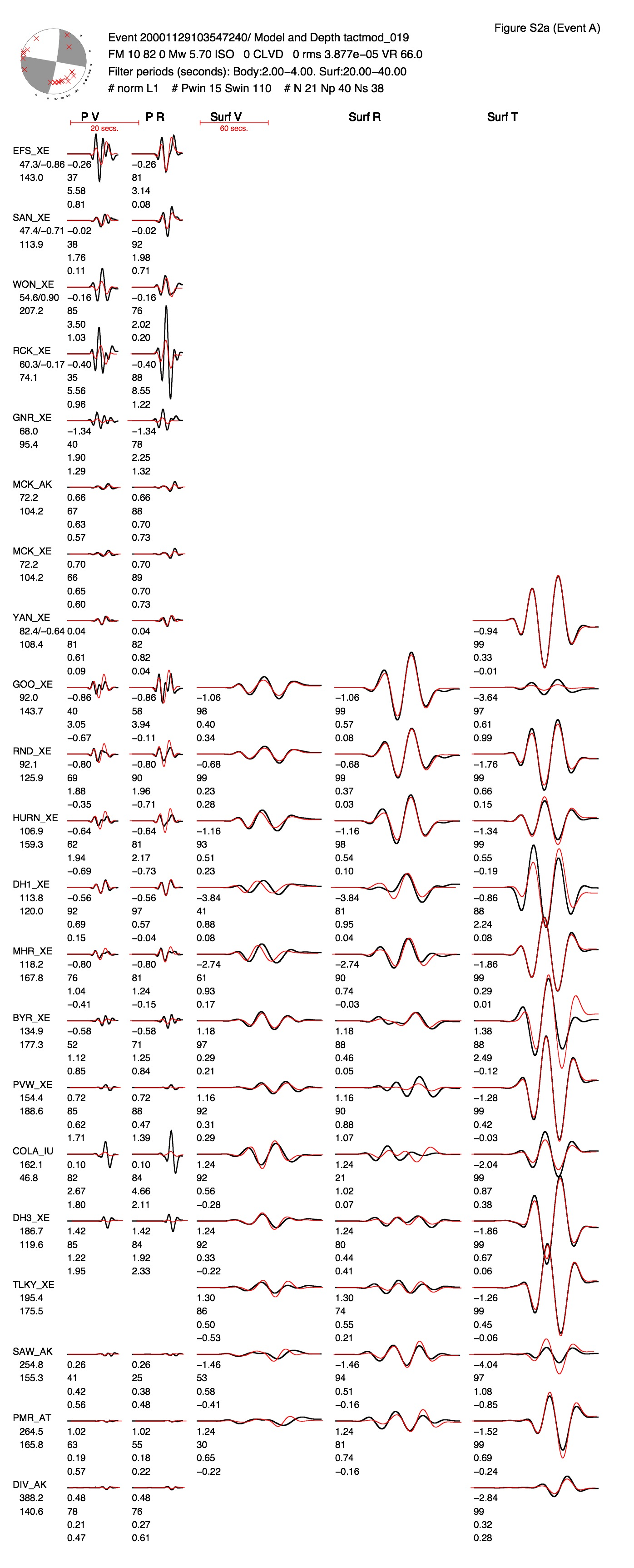
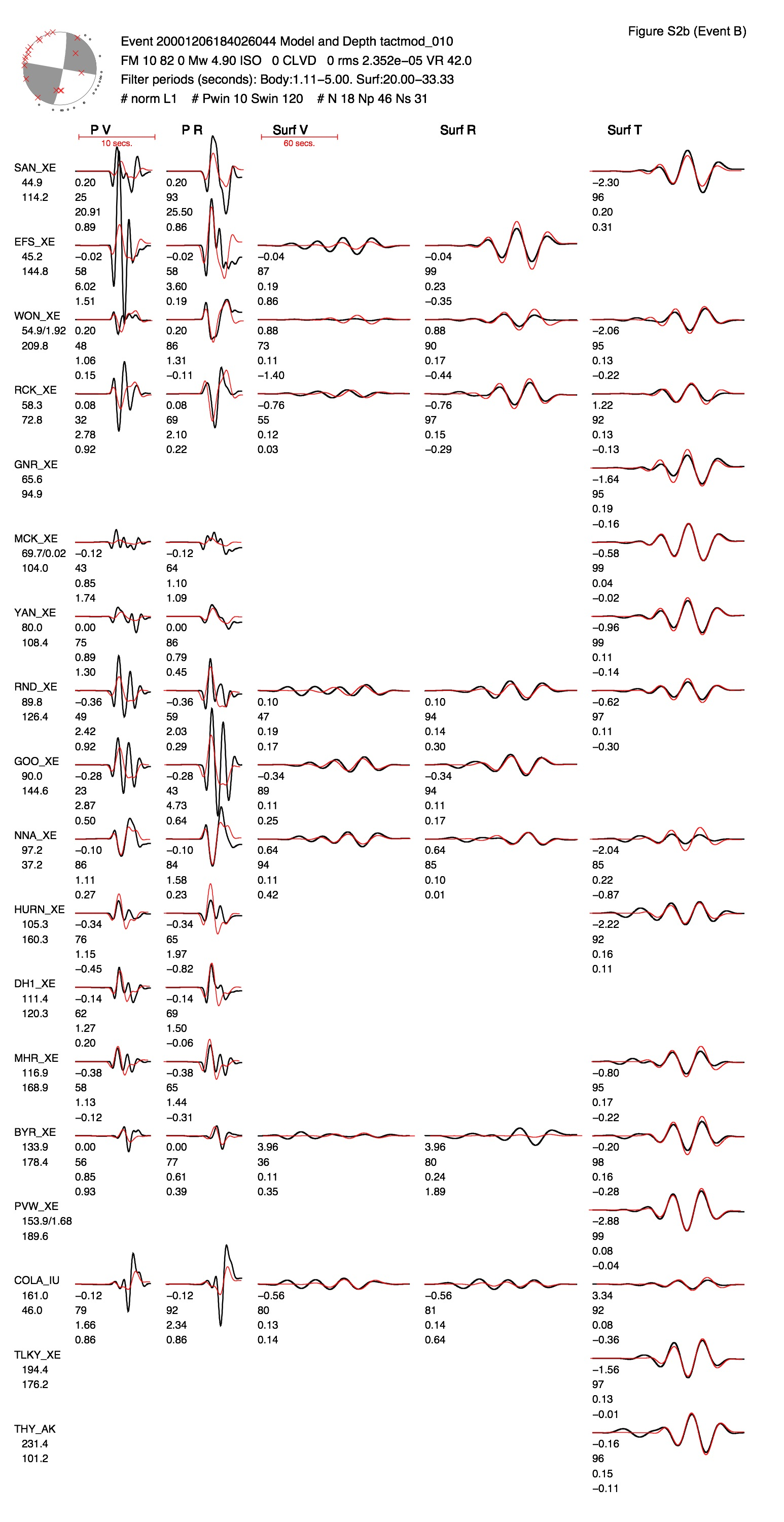
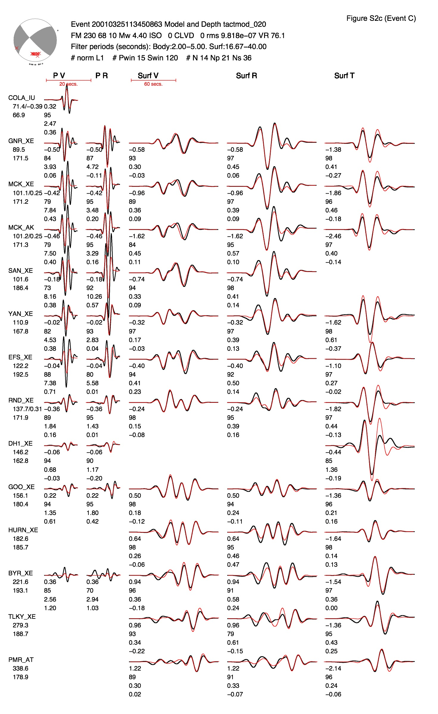
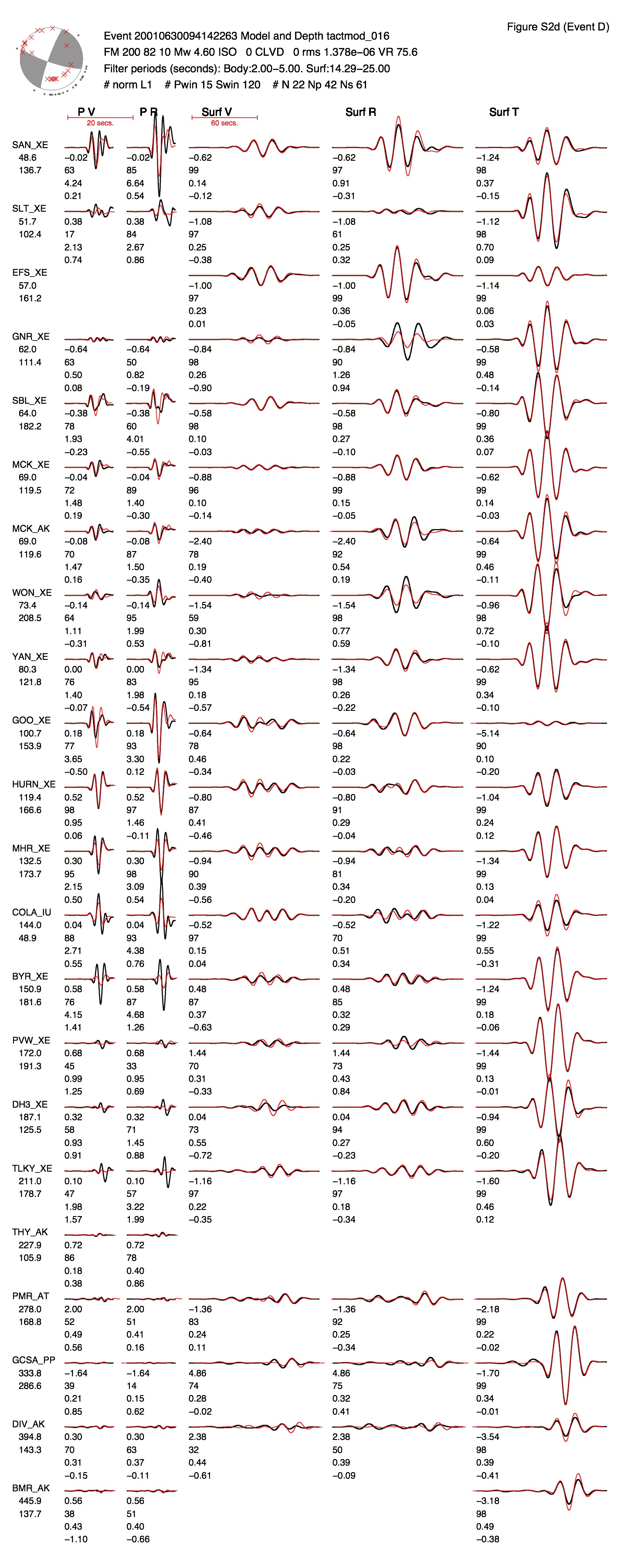
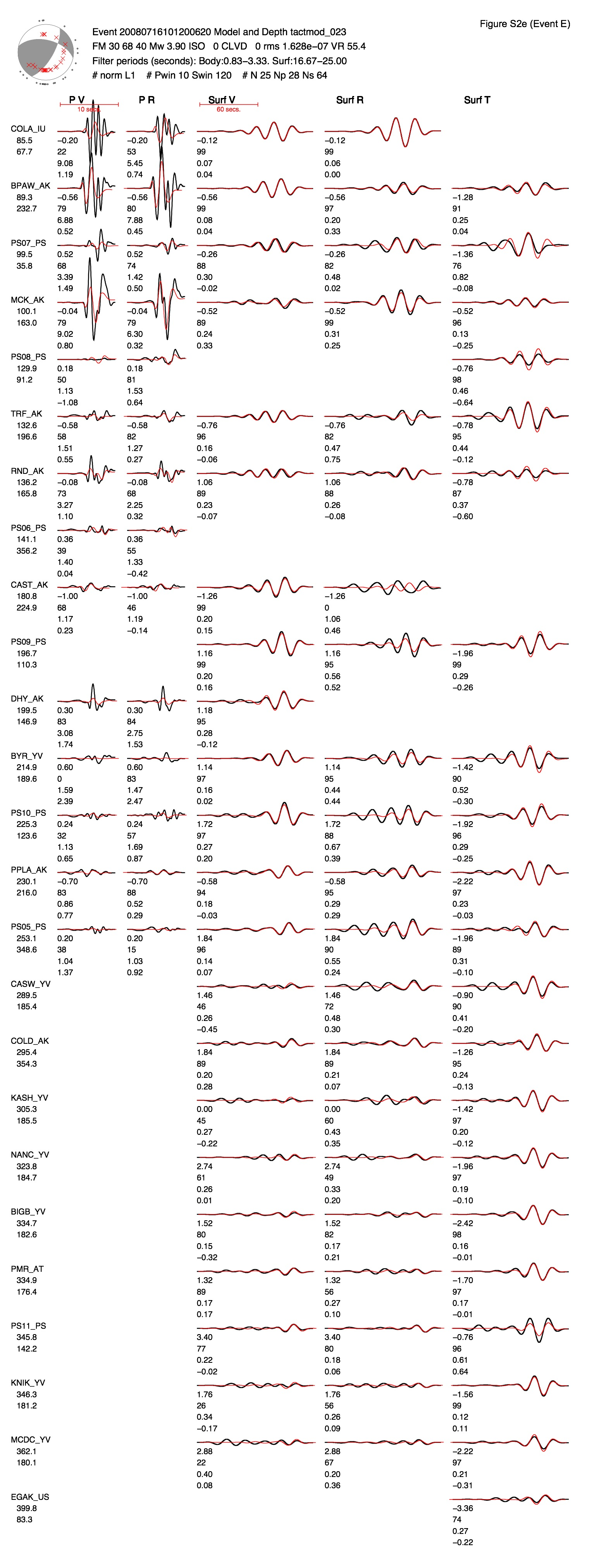
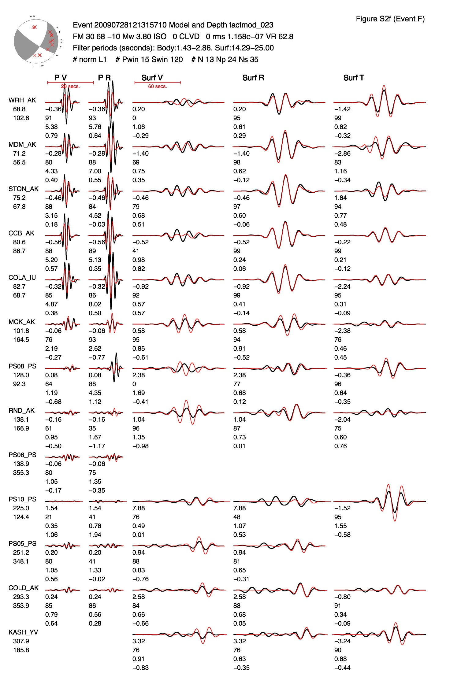
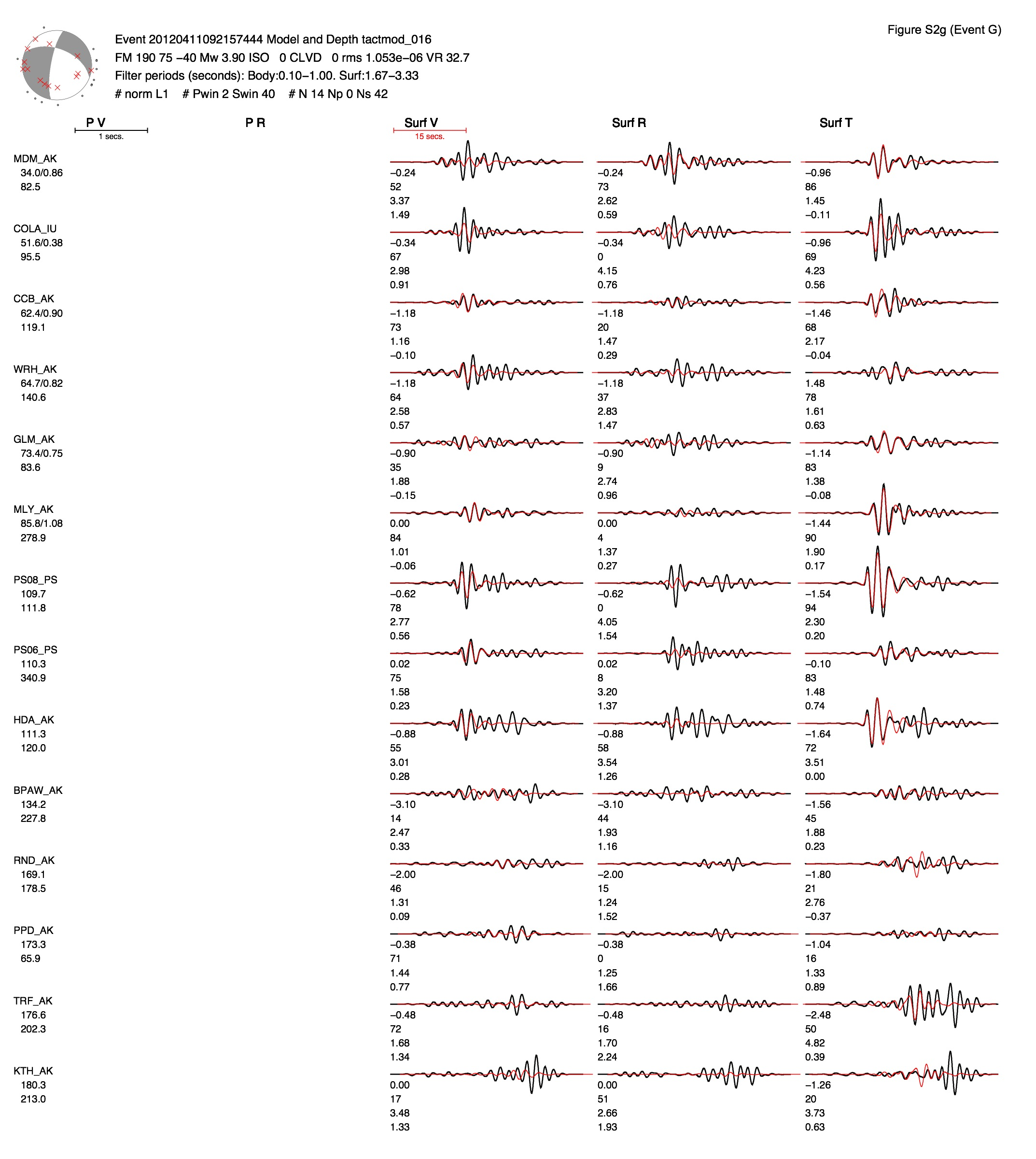
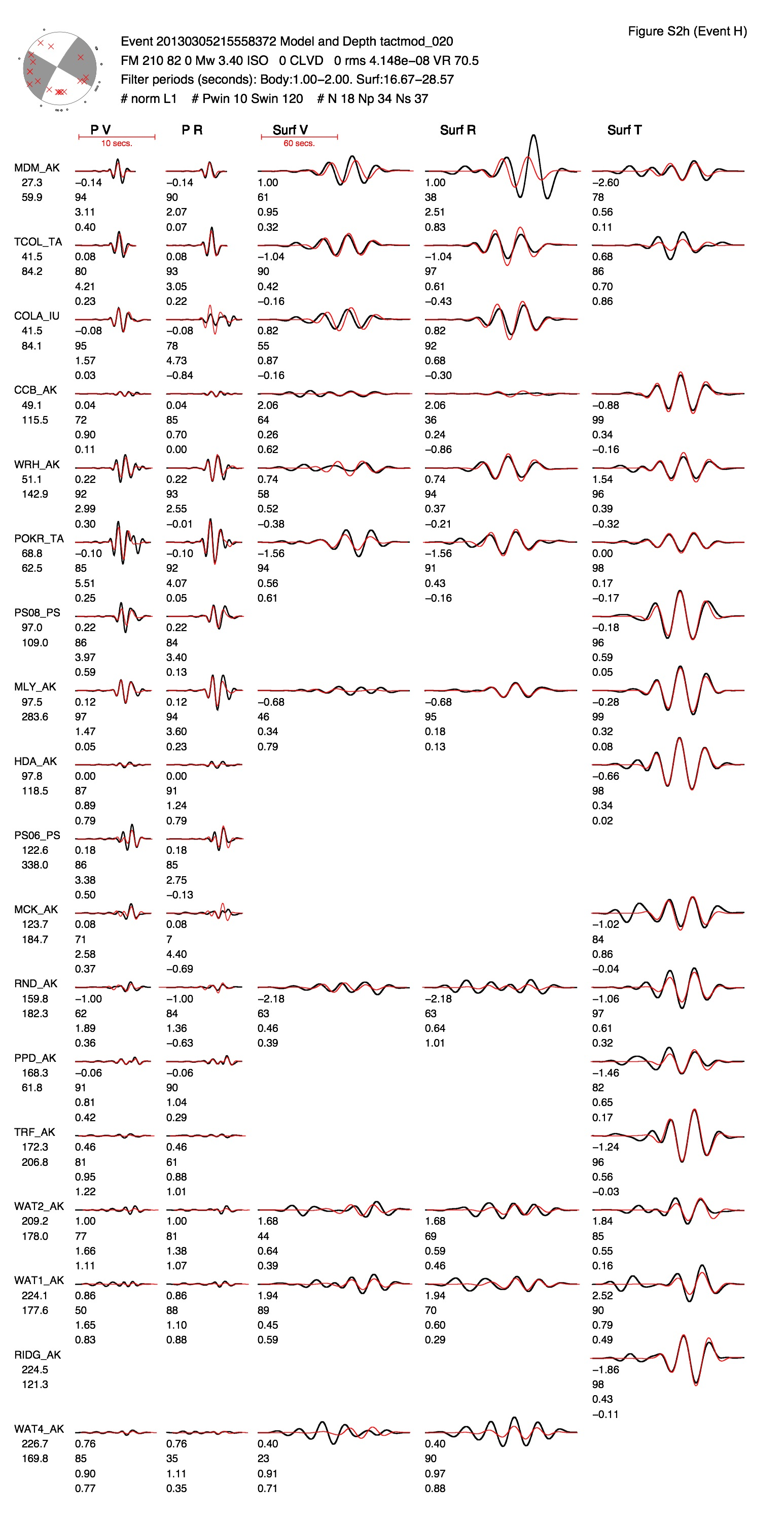
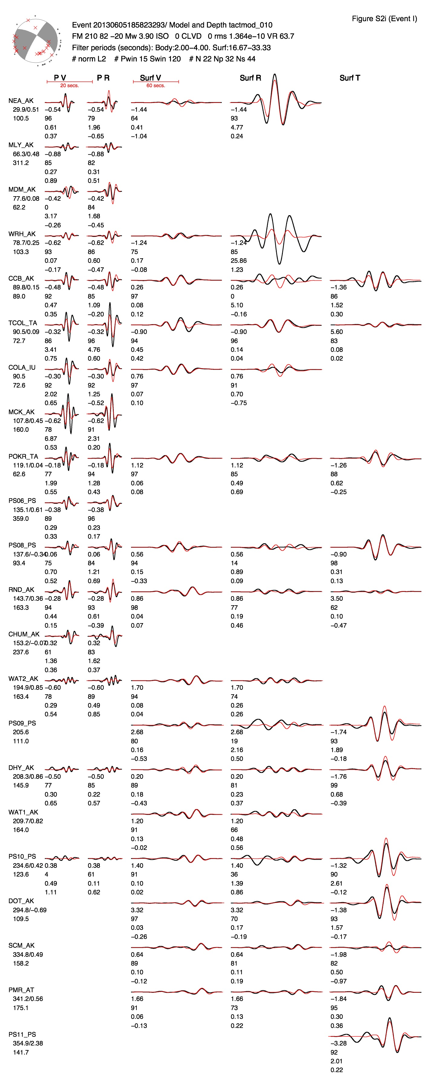
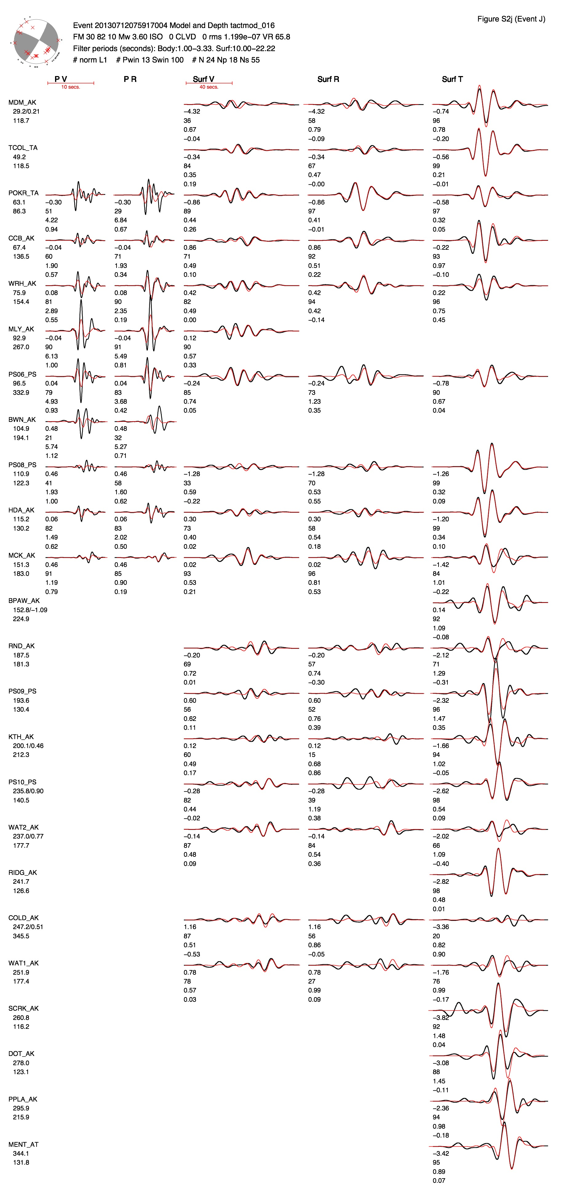
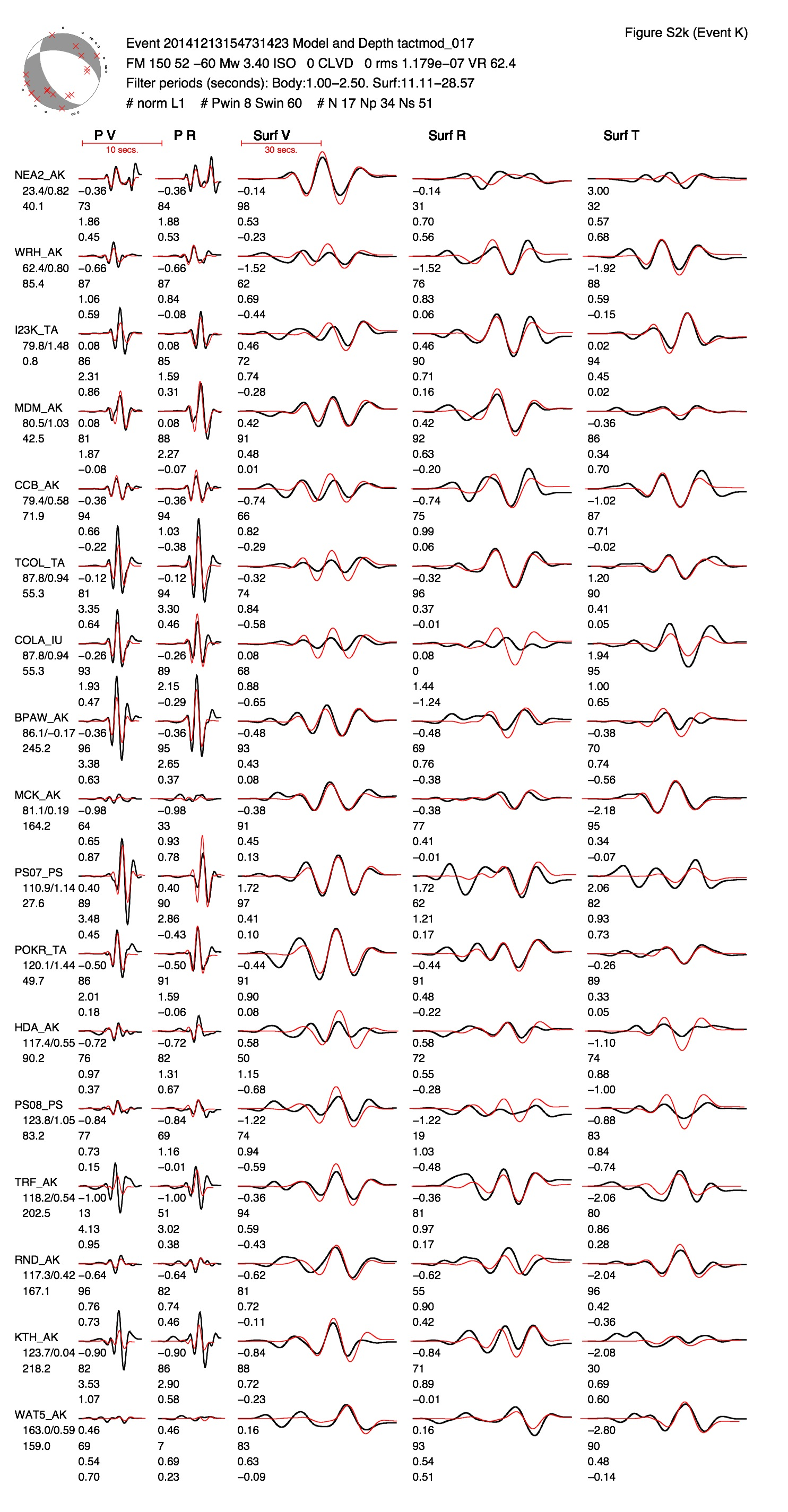
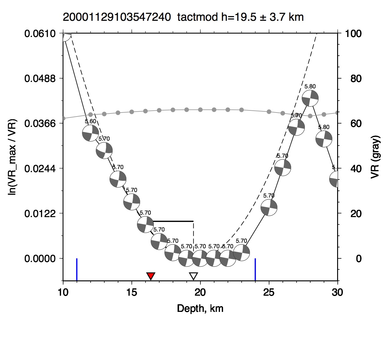
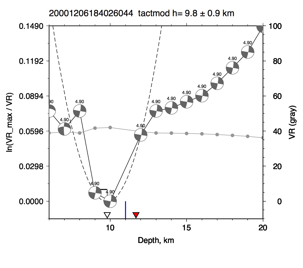
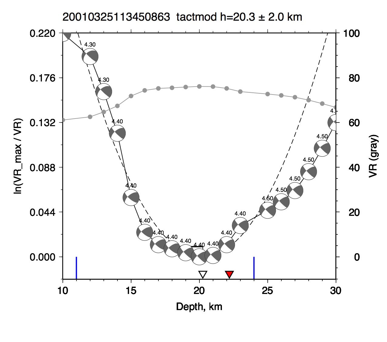
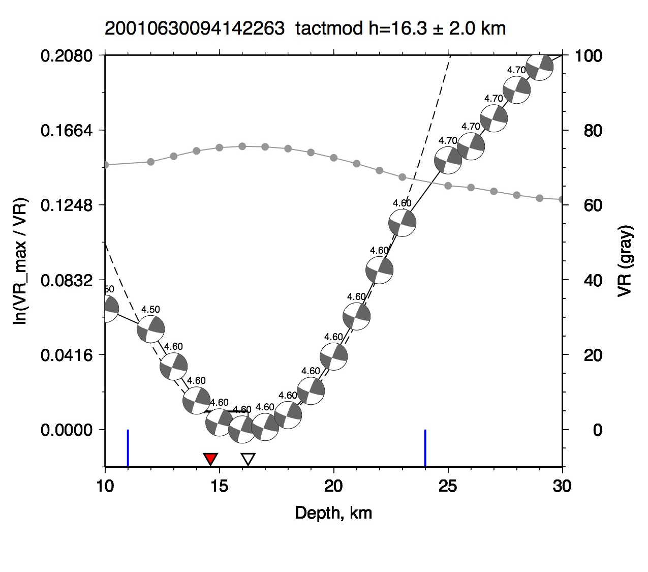
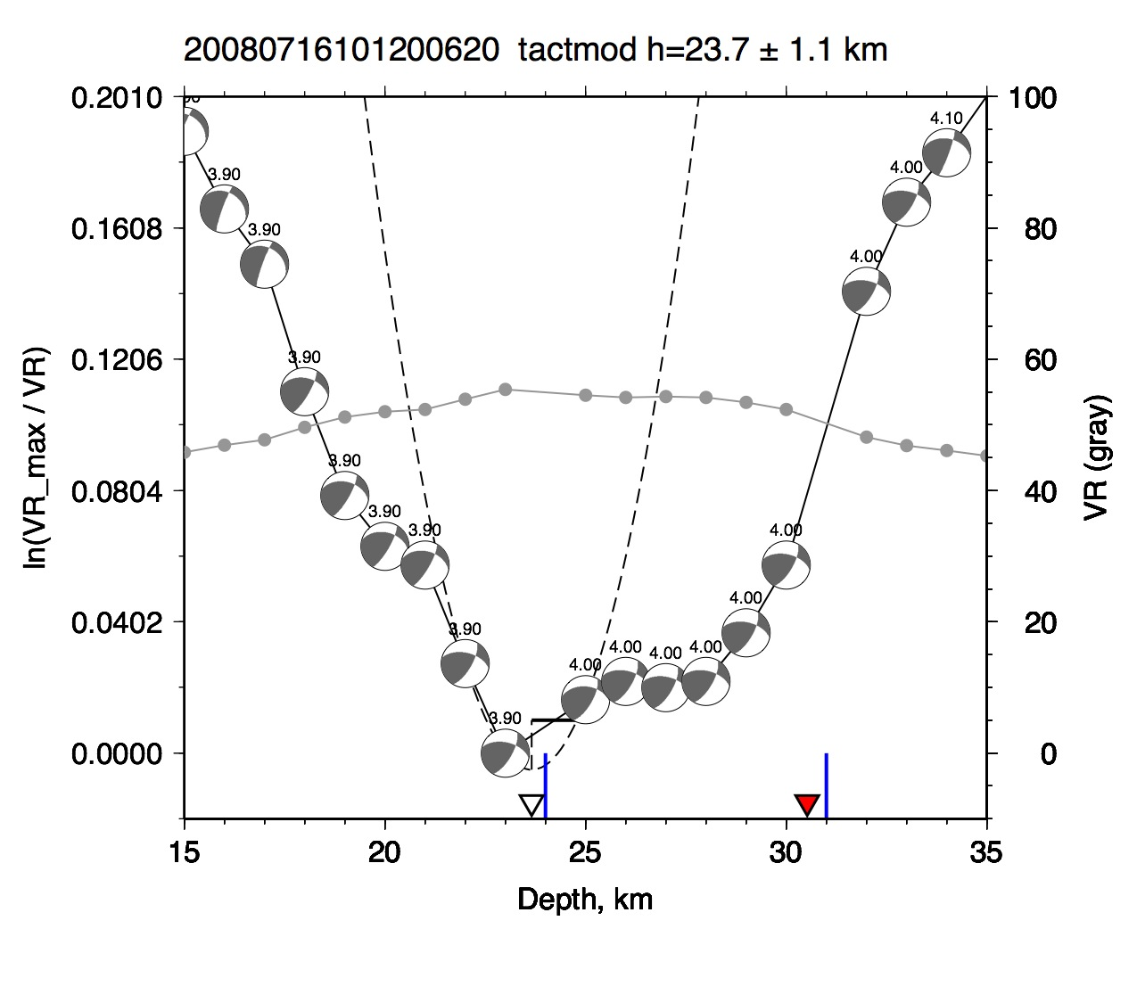
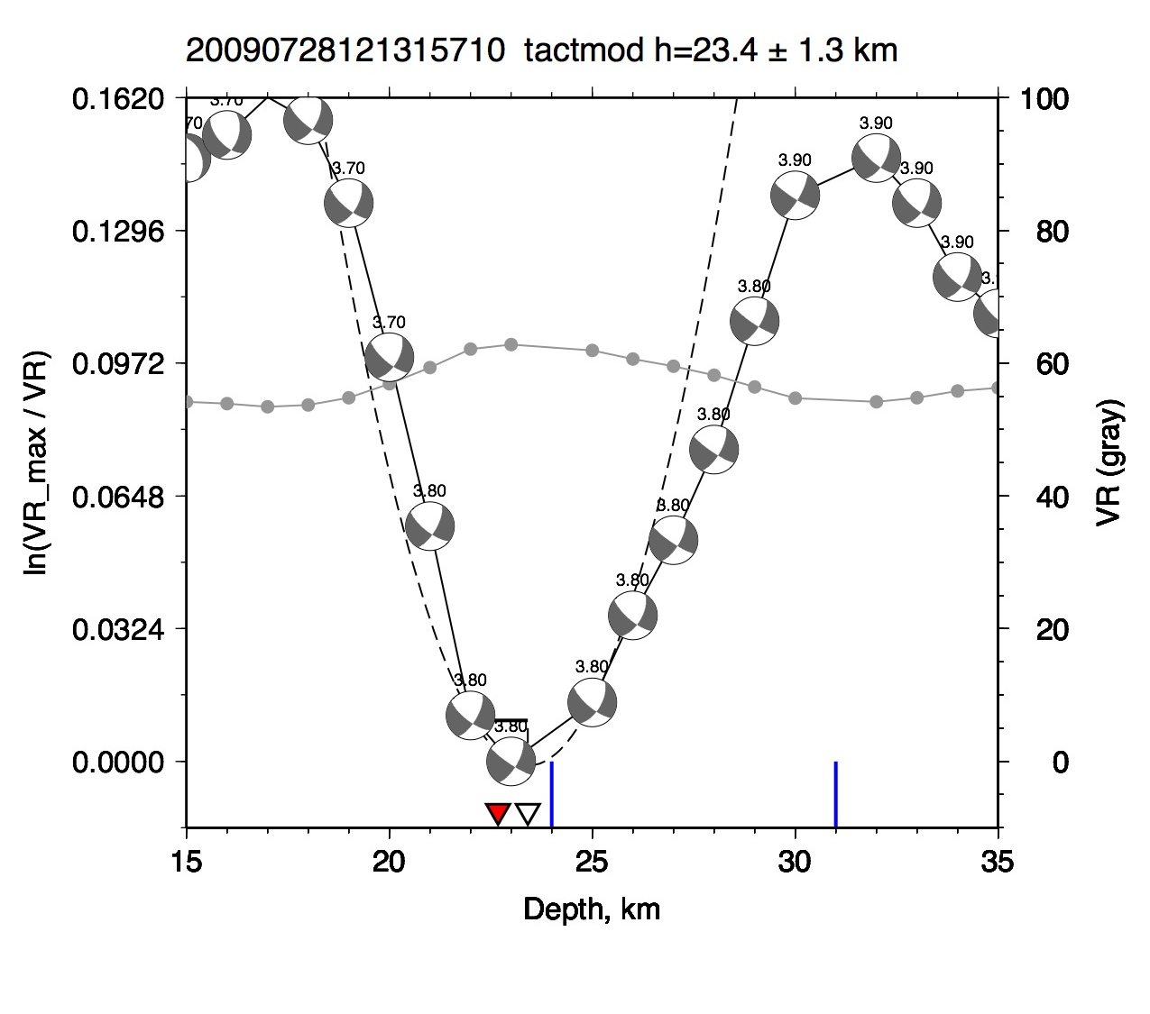
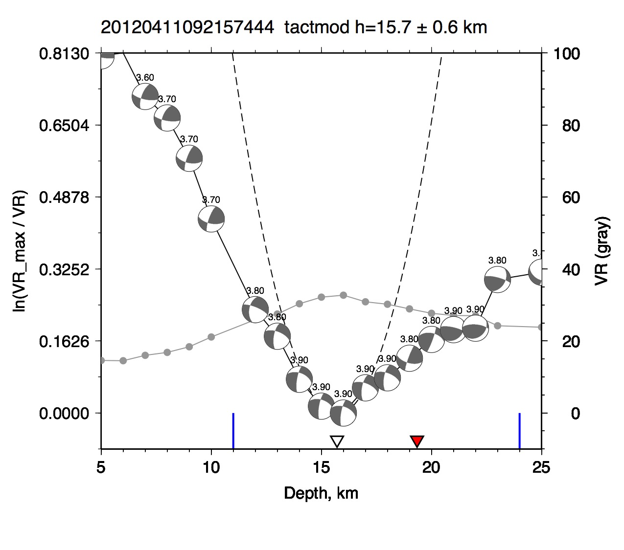
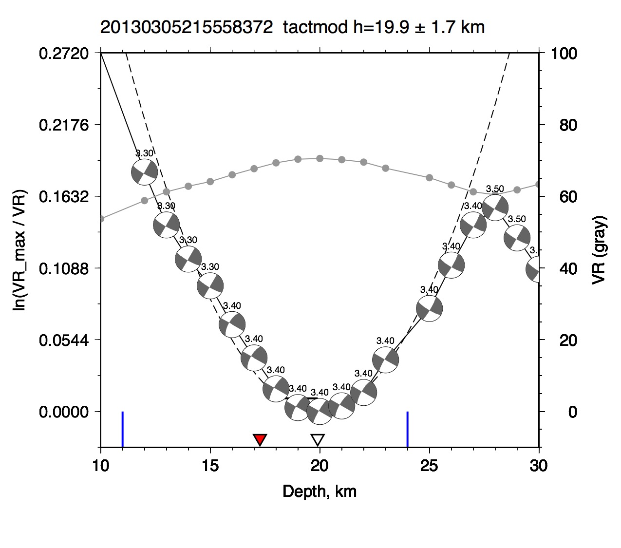
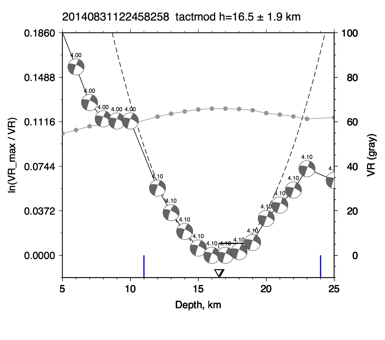
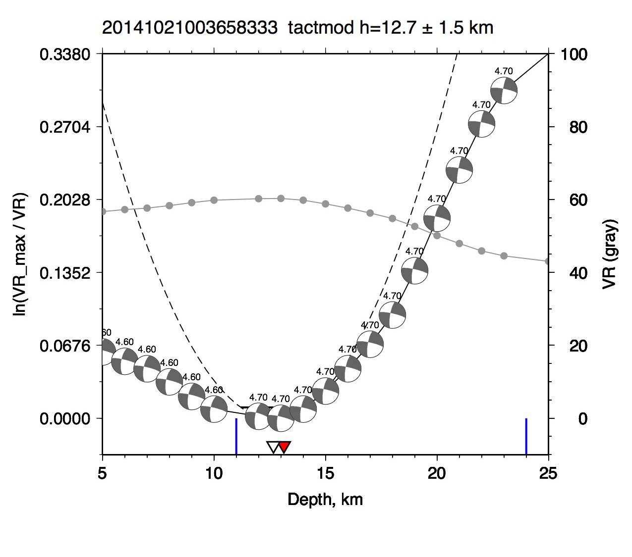
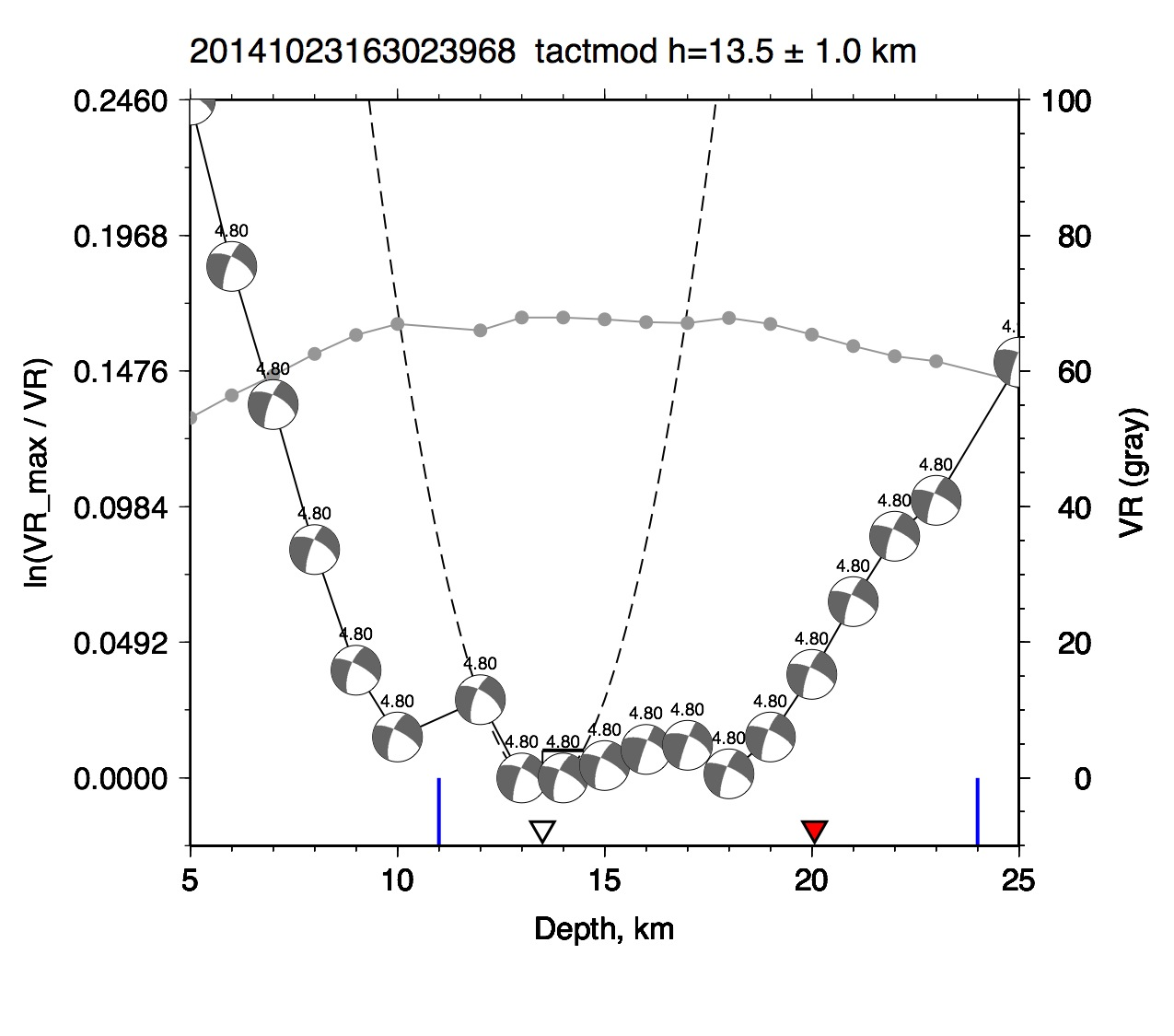
Figure S2a–o shows the waveform fits for the moment tensors listed in Table 1 and plotted in Figure 9, both in the main article. Figure S3a–o shows the corresponding best-fitting depths. The epicenters and origin times are taken from the Alaska Earthquake Center (AEC) catalog and are assumed to be fixed.

Seismicity Variations among the Subregions of the MFFZ

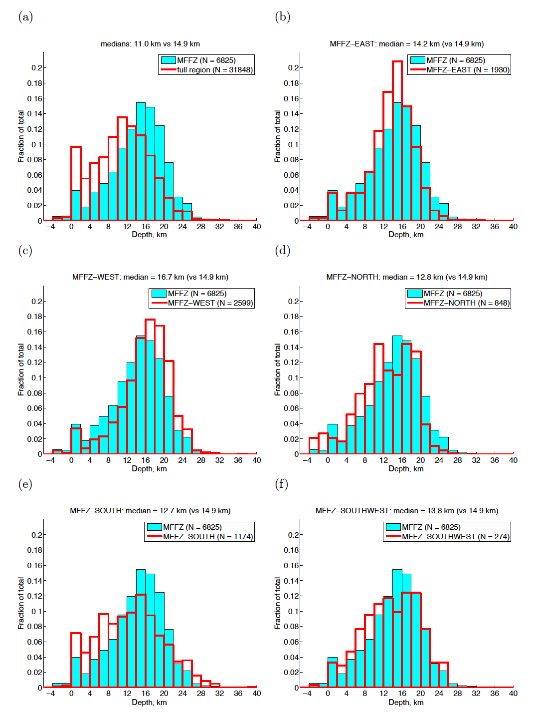
In Figures S4 and S5, we examine the differences in seismicity among the subregions of MMFZ. Figure S4 shows the b-value for each subregion. There is a clear difference between the b-values from subregions near the Nenana basin (west, east, and southwest; b ≈ 1.0) and the b-values north and south of the basin (b ≈ 0.8). The lower b-values in the north and south subregions suggest that larger-magnitude events in these regions will occur more frequently relative to smaller events. Figure S5 shows the distribution of depths of events within each subregion. Earthquakes in the west subregion are deeper than those in the east subregion (Fig. 6d in the main article), and earthquakes in the south subregion are more broadly spread over depths ranging from near the surface to 30 km.

The Fault Plane of the 1995 M_w 6.0 Earthquake

For the finite-slip inversion of the 1995 M_w 6.0 Minto earthquake, it is important to determine the fault plane for the inversion. Moment tensor solutions indicate either left-lateral faulting on a steep northeast–southwest-striking fault or right-lateral faulting on a steep northwest–southeast-striking fault. This choice is particularly important, because the event either occurred on the main fault of the fault zone or it occurred on a fault that is perpendicular to the fault zone, such as events L–O in Table 1 in the main article. We perform the finite slip inversion on both possible planes, as shown in Figure 11 of the main article and in Figure S7. The waveforms fits are significantly better for the northeast–southwest-striking plane (Fig. 11 in the main article).

We also examine the spatial distribution of aftershocks. We assume that aftershocks occurred on the fault plane. In this study, we relocate earthquake hypocenters using two different algorithms. The first algorithm is the joint hypocenter determination method, which was used in the study of Ratchkovski and Hansen (2002). The second algorithm is the waveform cross-correlation method used in producing the results in Figure 7 of the main article. Our objective is to estimate a best-fitting line (representing a vertical fault) through the epicenters from each catalog of aftershocks.

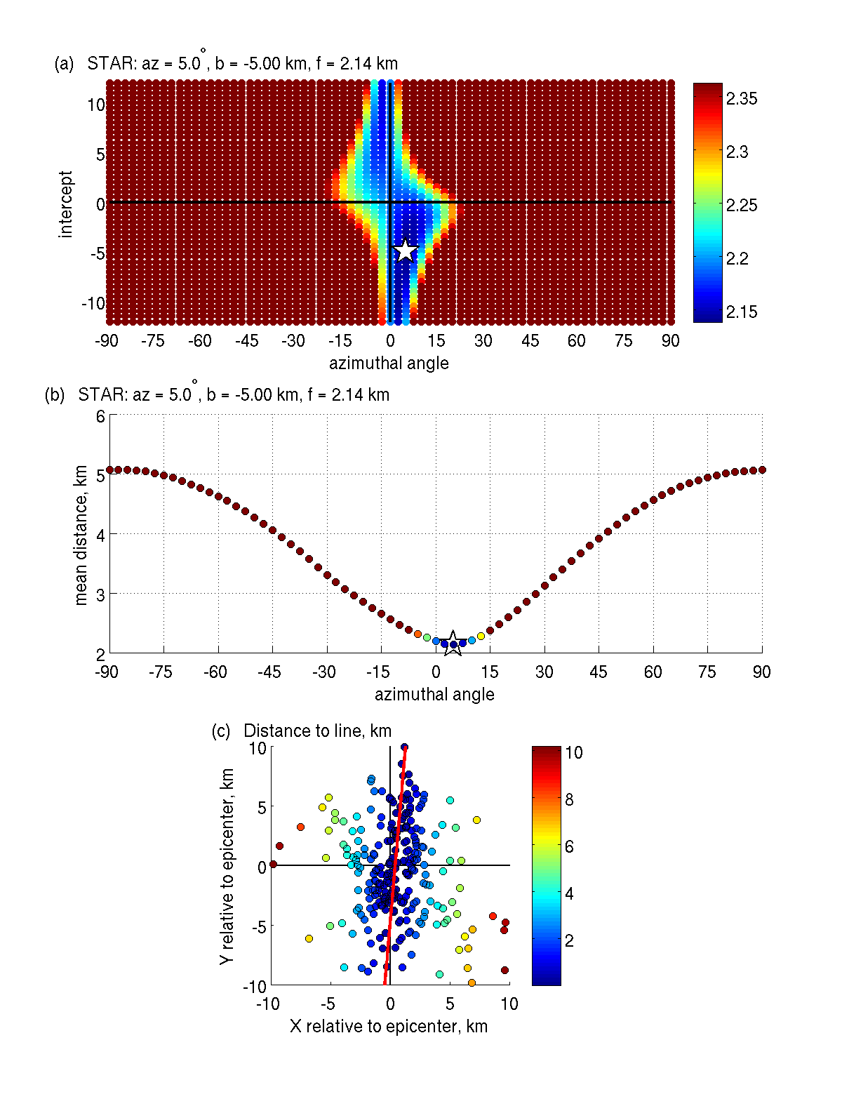
Figures S8–S10 show the analysis for the joint hypocenter determination method. These results are qualitatively similar to those presented in Ratchkovski and Hansen (2002, fig. 7). The hypocenters are diffuse but appear to be more concentrated on a north-northeast-striking plane. Figure S8 shows how we estimate the best-fitting line. Figure S8a shows the mean distance from all epicenters to each line characterized in a 2D model parameter space with the azimuthal angle of the line as the x variable and the y intercept as the y variable. The variation of the function provides a qualitative estimate for the uncertainty in the azimuthal angle of the line, which is the parameter of interest. (Note that the y intercept is not so useful for faults that strike near north, because small east–west shifts of the line correspond to large shifts in the y intercept.) Our misfit measure is based on the distance and represents an L1 (or robust) norm, which is less sensitive to outliers than an L2 norm that is based on a distance-squared measure. Figure S8a reveals that the best-fitting line has an azimuth ranging from −10° to 15°, with the optimum value of 5°.

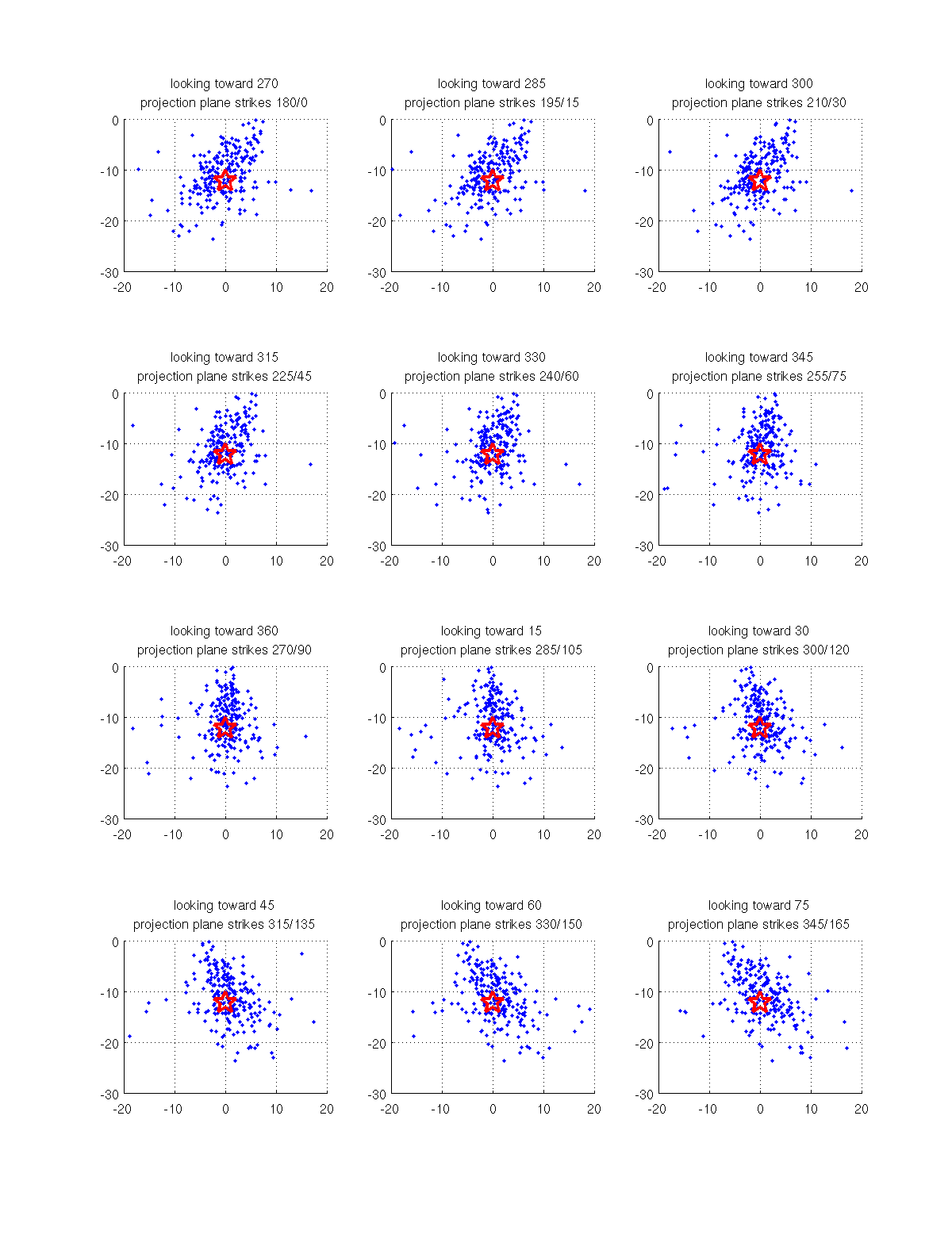
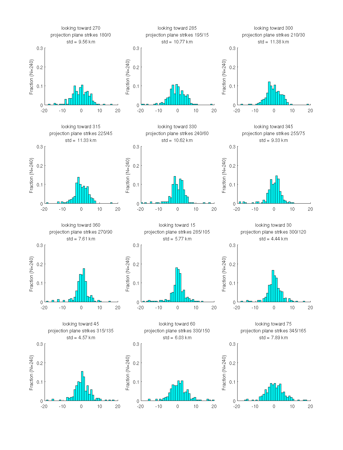
Figure S9 shows the aftershock seismicity projected onto vertical planes that contain the epicenter. The top-center subplot, where the projection plane strikes 195° (15°), is similar to the plot in Ratchkovski and Hansen (2002, fig. 7) labeled as SSW–NNW. Both plots show a pattern of shallower aftershocks to the north and deeper aftershocks to the south. Ratchkovski and Hansen (2002, fig. 7) identified diffuse aftershocks beneath 15 km; this pattern is not as apparent in our reanalysis in Figure S9. Figure S10 is a supplemental plot of the data in Figure S9. If all events were on a vertical fault plane, then the histogram would be a single peak at zero. We see that the histograms are narrower when looking in the direction 0° to 30°.

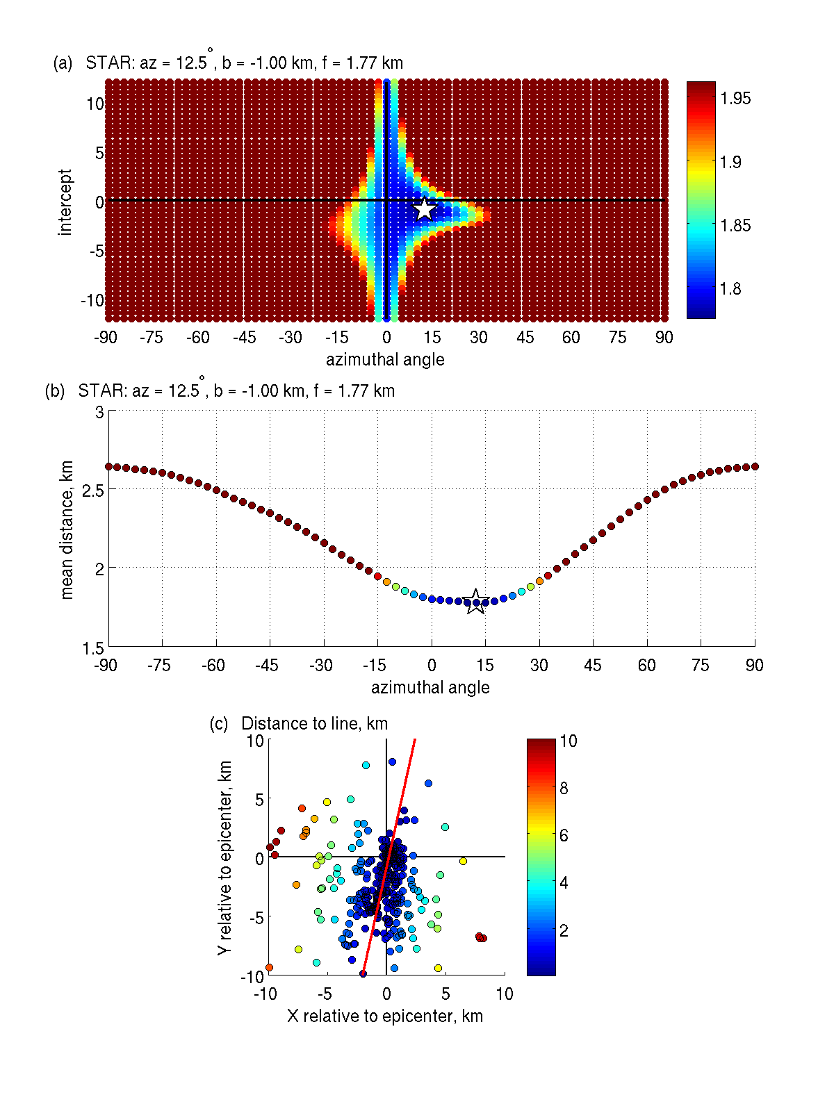
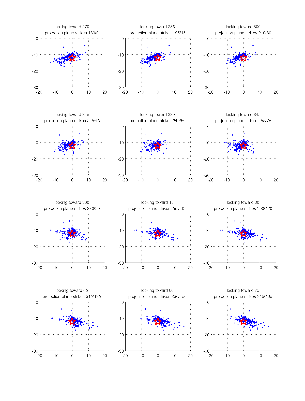
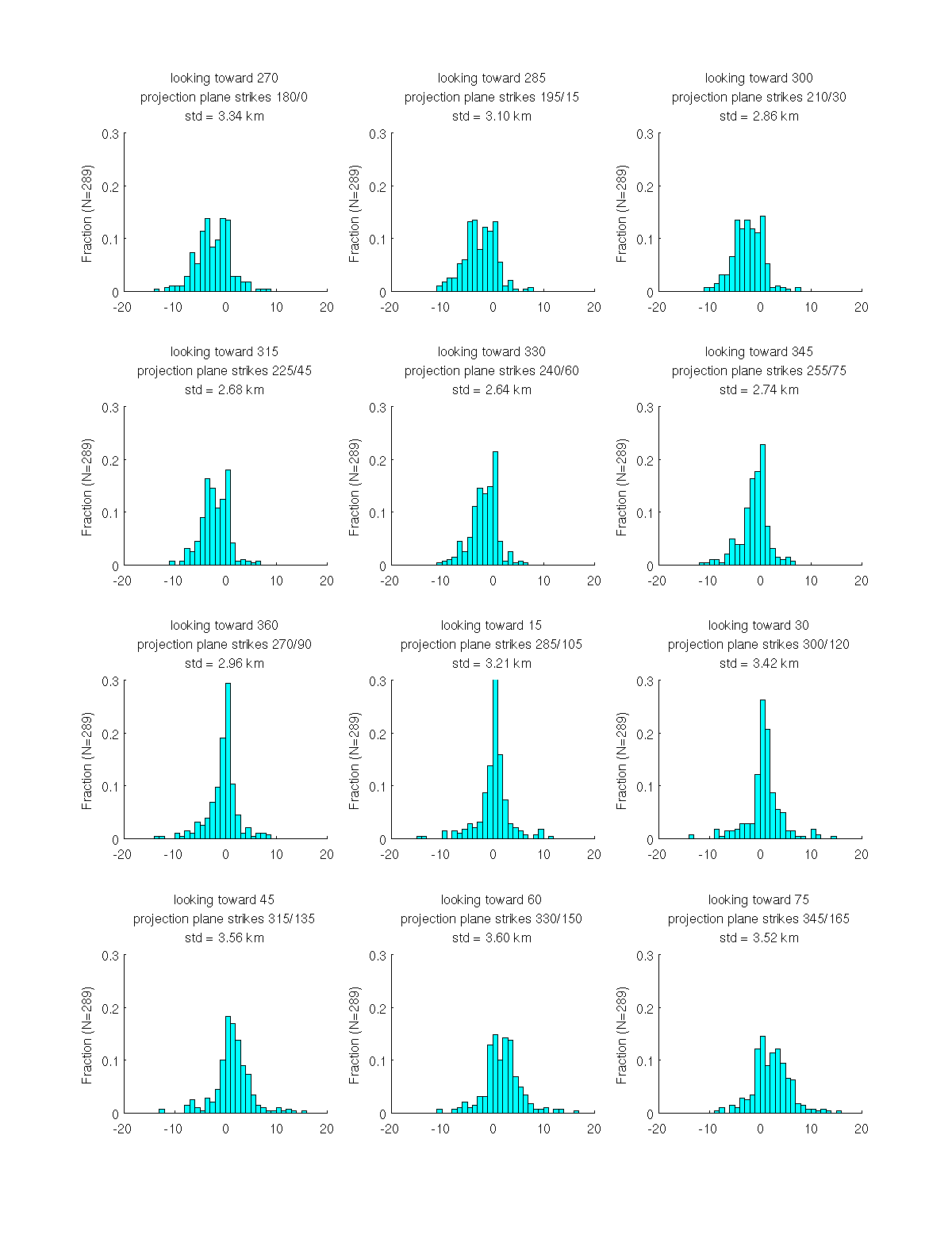
Figures S11–S13 show the same analysis for the aftershock catalog produced from waveform cross correlation. In this case we obtain a best-fitting line with azimuth 12.5°. The results in Figure S12 show the same pattern as in Figure S9: shallow aftershocks in the north and deeper aftershocks in the south. The depths range from 8 to 18 km and are much tighter in Figure S12 than in Figure S9.

---

Table

Table S1. Moment tensor solutions from this study. In this ASCII text file, the moment tensor is provided as six M_ij entries in units of N · m. The basis is the same as the Global Centroid Moment Tensor convention: up-south-east. These entries are listed with the highest precision. Other quantities derived from M_ij are also shown but are not listed with the highest precision.

---

Figures

Figure S1. Log-scaled crustal seismicity rate for central Alaska. The parameters from the AEC seismicity catalog are 1990-01-01 to 2015-01-01, M ≥ 0, and depth ≤40 km, in order to eliminate slab events. Fault zones: MFFZ, Minto Flats fault zone; FSZ, Fairbanks seismic zone; and SSZ, Salcha seismic zone. This is an expanded version of Tape et al. (2013, fig. S4). Active faults from Koehler et al. (2012) are plotted as black lines. The magnitude of catalog completeness varies from about M_c = 0.5 to 1.5 over this region (Ruppert et al., 2008, plate 1), so some lack of seismicity could be due to the higher completeness magnitudes.

Figure S2a, b, c, d, e, f, g, h, i, j, k, l, m, n, and o. Waveform fits for the moment tensor inversions in this study. Figure S2a–o corresponds with events A–O listed in Table 1 in the main article. A subset of waveform fits for Figure S2a (event A) is shown in Figure 8 in the main article. The black lines are the observed waveforms; the red lines are the synthetic waveforms computed using the 1D model tactmod (Beaudoin et al., 1992; Ratchkovski and Hansen, 2002). The waveforms are fit separately within five time windows: P-wave vertical component (PV), P-wave radial component (PR), Rayleigh-wave vertical component (Surf V), Rayleigh-wave horizontal component (Surf R), and Love-wave transverse component (Surf T). At the far left in each row is the station name, source–station distance in kilometers, and station azimuth in degrees. Below each pair of waveforms are four numbers: the cross-correlation time shift between data and synthetics, the cross-correlation value, the percent of the misfit function represented by the waveform pair, and the amplitude ratio between waveforms, ln(A_obs/A_syn), in which A is the maximum value of the waveform within the time window. For example, Pwin 15 Swin 110 # N 21 Np 40 Ns 38 indicates that the (reference) P-window is 15 s long, the surface-wave window is 110 s long, there are 21 stations with at least one waveform, 40 P windows were used, and 38 surface-wave windows were used.

Download/View: Figure S2a-o Combined [PDF; ~13 MB].

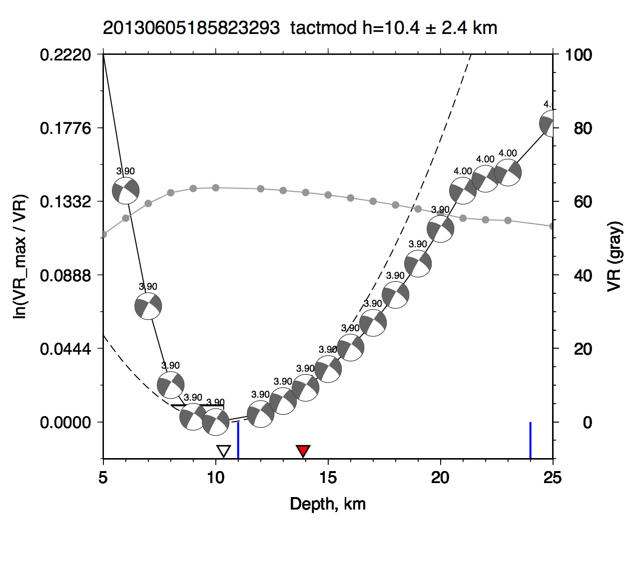
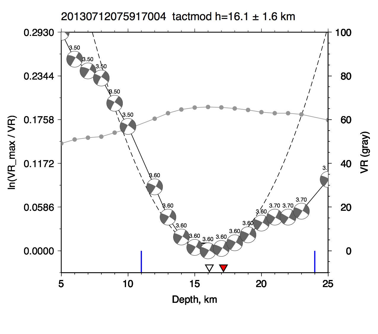
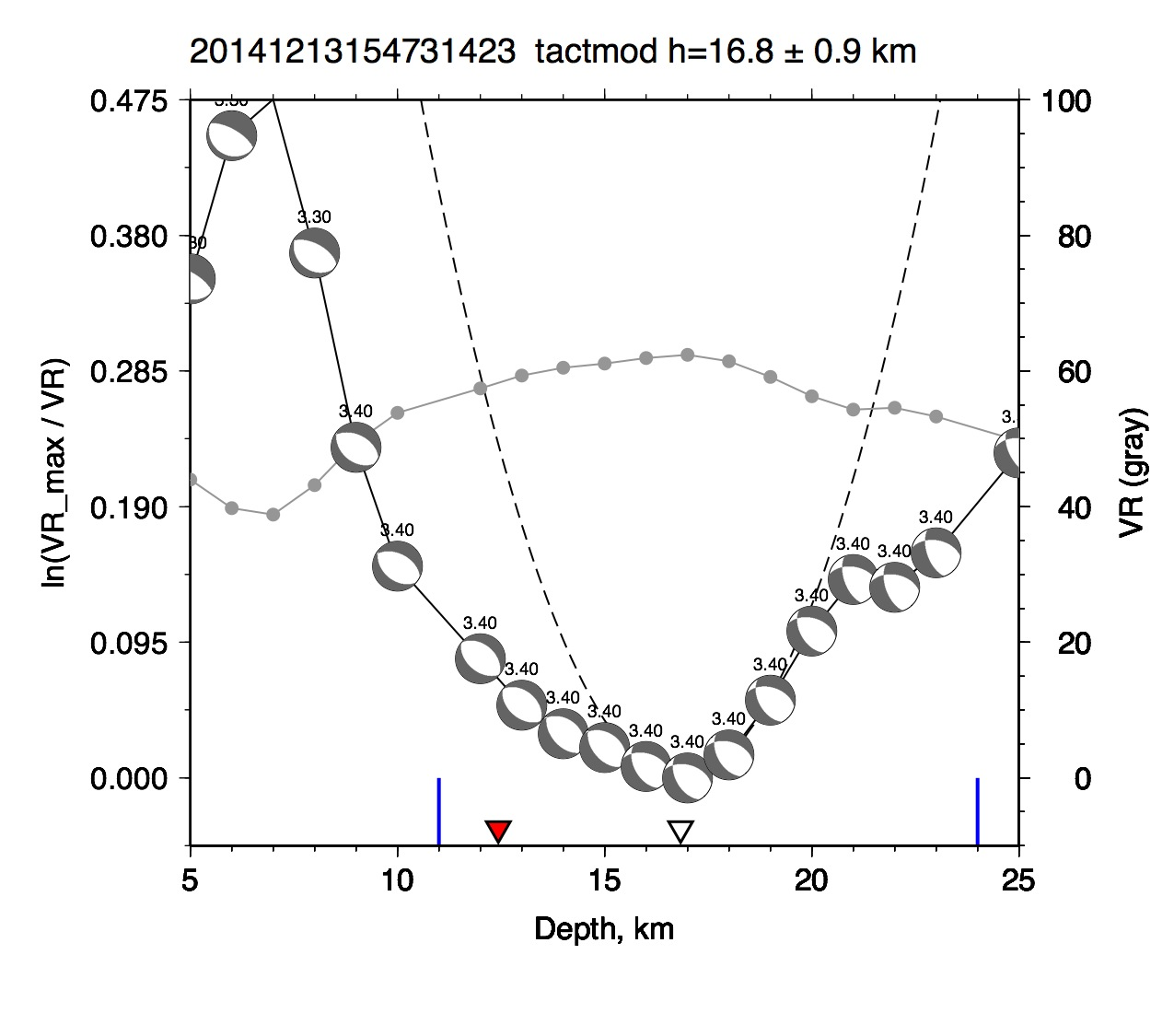
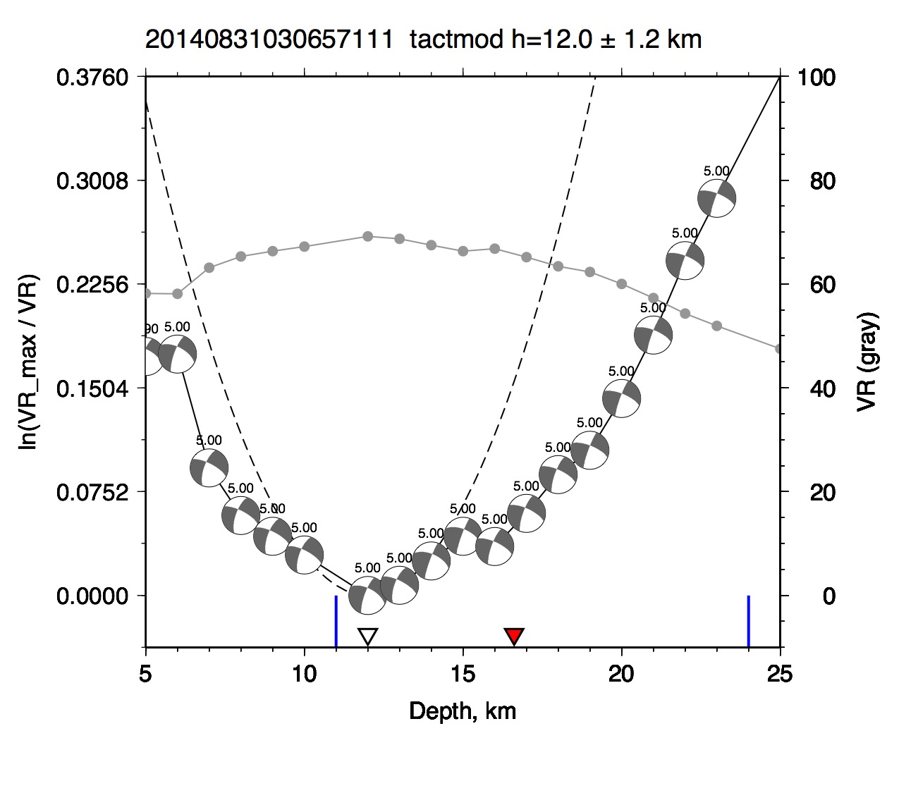
Figure S3a, b, c, d, e, f, g, h, i, j, k, l, m, n, and o. Best-fitting depths for the moment tensor inversions in this study. Figure S3a–o corresponds with events A–O listed in Table 1 in the main article. The red triangle marks the AEC catalog depth, and the white triangle marks the depth obtained from the moment tensor inversion. The blue lines on the x axis mark the layer boundaries in the 1D model (tactmod) used in the moment tensor inversions. The plot shows the variance reduction (VR, gray curve), with the scale on the right. On the left is the variance reduction relative to the minimum variance reduction. The depth uncertainty is calculated based on the depth at which the variance reduction is 0.10 worse than at the best solution.

Download/View: Figure S3a-o Combined [PDF; ~1 MB].

Figure S4. Frequency–magnitude distributions for subregions of the MMFZ. The subregions are shown in Figure 4b in the main article. The date range of seismicity is 1990-01-01 to 2015-01-01; the total number of events (nevents) is 6825. The b-value is estimated from a best-fitting line over the magnitude interval M 1.5–3.5: (a) all five subregions (b = 0.87) (same as Fig. 6b in the main article), (b) east subregion (b = 1.01), (c) west subregion (b = 0.93), (d) north subregion (b = 0.79), (e) south subregion (b = 0.78), and (f) southwest subregion (b = 1.04). The a-value from the best-fitting line is the y-intercept for the log-scaled coordinates. The first value is for the cumulative distribution, and the value in parentheses is for the incremental distribution.

Figure S5. Comparison of depths among MFFZ subregions. The subregions are shown in Figure 4b of the main article. The date range of seismicity is 1990-01-01 to 2015-01-01. (a) Comparison between the five subregions of the MFFZ (e.g., Fig. 4b in the main article) and the full region in Figure 2a (same as Fig. 6c in the main article). Comparisons between the MFFZ and (b) the east subregion, (c) the west subregion, (d) the north subregion, (e) the south subregion, and (f) the southwest subregion.

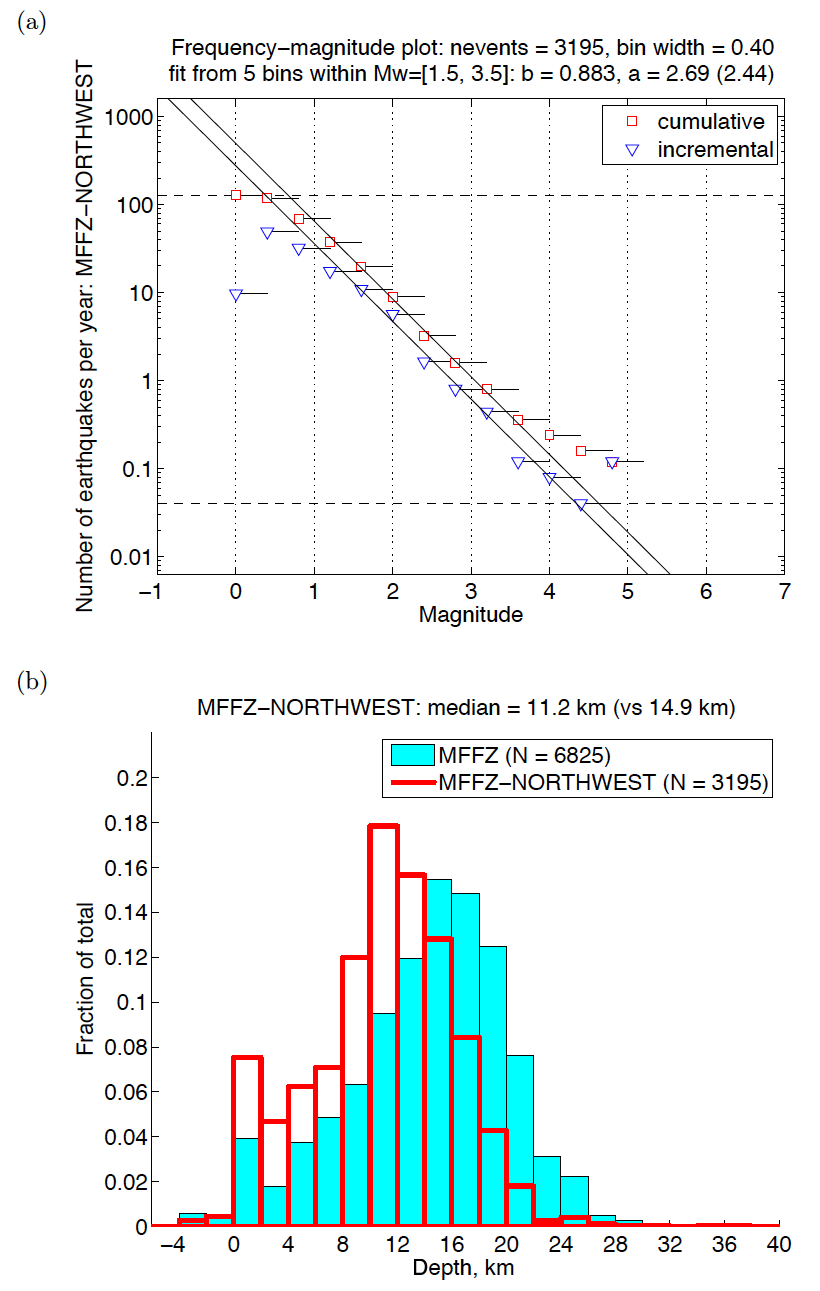
Figure S6. Seismicity analysis for the northwest subregion (Fig. 4b in the main article), which is not considered part of the MFFZ. For completeness, we include this for comparison with the other subregions in Figures S4 and S5: (a) the frequency–magnitude distribution (b = 0.88) and (b) comparison between depths in the northwest subregion (median 11.2 km) and the depths within the (adjacent) MFFZ (median 14.9 km).

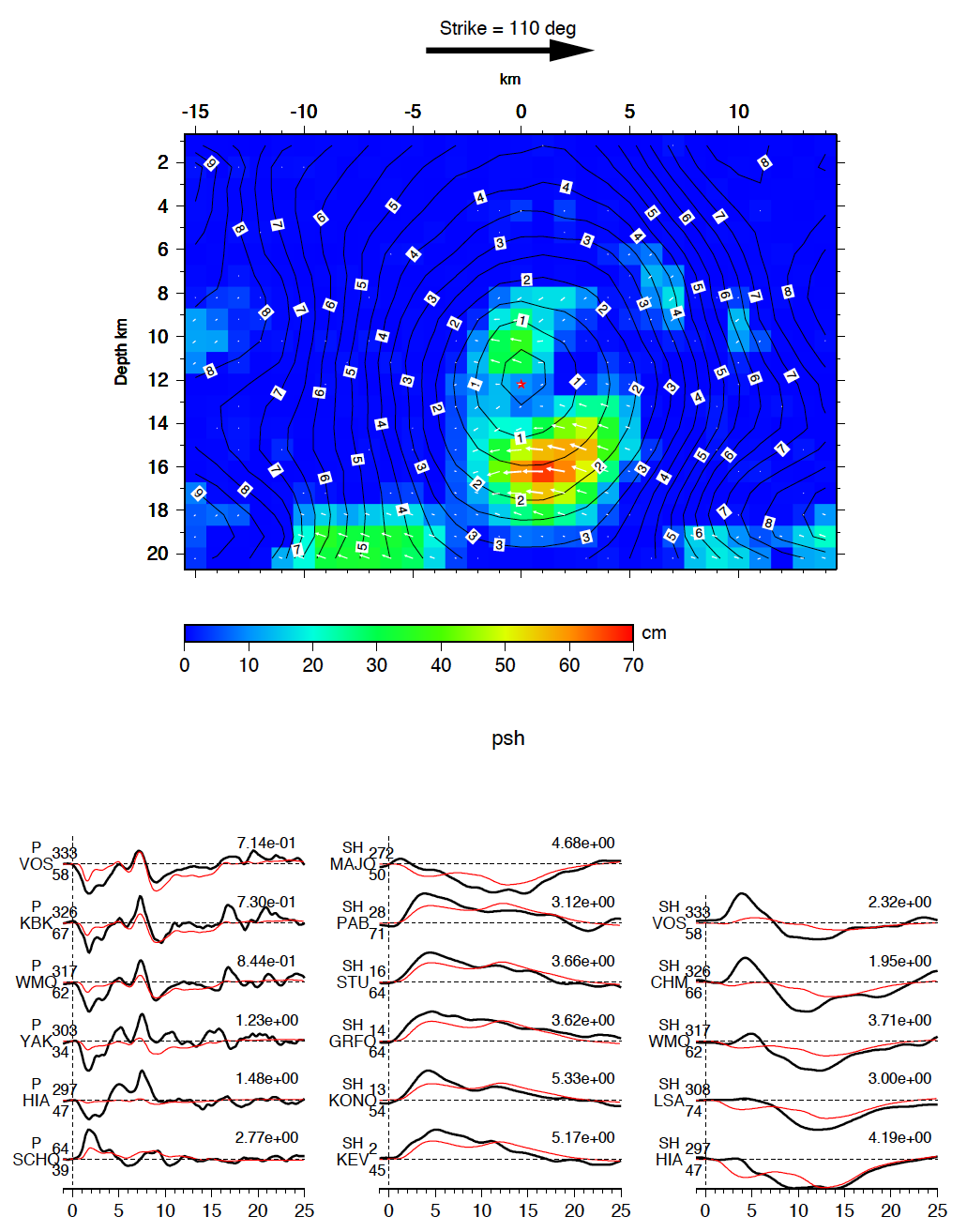
Figure S7. Finite slip inversion for the 1995 M_w 6.0 Minto earthquake. Here we have used the auxiliary plane (strike 110°, dip 90°, rake 170°) to the one shown in Figure 11 of the main article (strike 200°, dip 80°, rake 0°). Here the poor fits to the data support our interpretation that this is not the fault plane. (a) Cross section of the slip distribution. The direction of the view is toward the north (azimuth 20°). The red star indicates the hypocenter, the color denotes the slip amplitude (see color scale), and black contour lines indicate the rupture time in seconds. (b) The sum of the moment rate functions for all subfaults, with each moment rate function time-shifted by its onset time. For each comparison, the value above the beginning of the trace is the station azimuth relative to the epicenter, and the value below is epicentral distance. The value above the end of the trace is the observed peak amplitude in μm/s, which is used to normalize the synthetic and observed seismograms.

Figure S8. Estimating a best-fitting line for aftershock epicenters of the M_w 6.0 earthquake. The aftershocks were relocated using a joint hypocenter determination method (e.g., Ratchkovski and Hansen, 2002). (a) Mean distance in kilometers from all epicenters to each line characterized by its azimuthal angle (x coordinate) and its intercept (y coordinate). The azimuthal angle of the best-fitting line is constrained between −10° and 15°. (b) Cross section of (a) for intercept fixed at b = −5.00 km. (c) Epicenters are colored by distance (in km) to the best-fitting (red) line.

Figure S9. Double-difference relocations of aftershocks of the 1995 M_w 6.0 earthquake, projected onto vertical planes with varying strike. The x-value is the horizontal distance from the mainshock epicenter. The y-value is height above sea level.

Figure S10. Histograms of the plots in Figure S9. Clustering is broadest when looking at the fault plane and narrowest when looking in the direction of the strike of the fault plane.

Figure S11. Estimating a best-fitting line for aftershock epicenters of the M_w 6.0 earthquake. The aftershocks were relocated using waveform cross correlation, as described in the main article (e.g., Fig. 7). (a) Mean distance in kilometers from all epicenters to each line characterized by its azimuthal angle (x coordinate) and its intercept (y coordinate). The azimuthal angle of the best-fitting line is constrained between −5° and 25°. (b) Cross section of (a) for the intercept fixed at b = −1.00 km. (c) Epicenters colored by distance (in km) to the best-fitting line, which is plotted in red.

Figure S12. Double-difference relocations of aftershocks of the 1995 M_w 6.0 earthquake, projected onto vertical planes with varying strike.

Figure S13. Histograms of the plots in Figure S12. Clustering is broadest when looking at the fault plane and narrowest when looking in the direction of the strike of the fault plane.

---

[ Back ]