This electronic supplement contains figures illustrating seismograms, process procedure, imaged reflectors, and resolved velocity structure for six broadband stations and one short-period station. Selected earthquake waveforms from all broadband stations and one short-period station of the Cooperative New Madrid Seismic Network (CNMSN) were examined and analyzed to image common reflectors and to resolve velocity structure for shallow crust (~5 km) in the upper Mississippi embayment. Examples of seismograms, process procedures, and results for a broadband station (HALT) are shown and described in the main article. Examples from the other remaining six broadband stations, GLAT, GNAR, HENM, LNXT, LPAR, PEBM, and a short-period station, MORT, are included in this supplement.
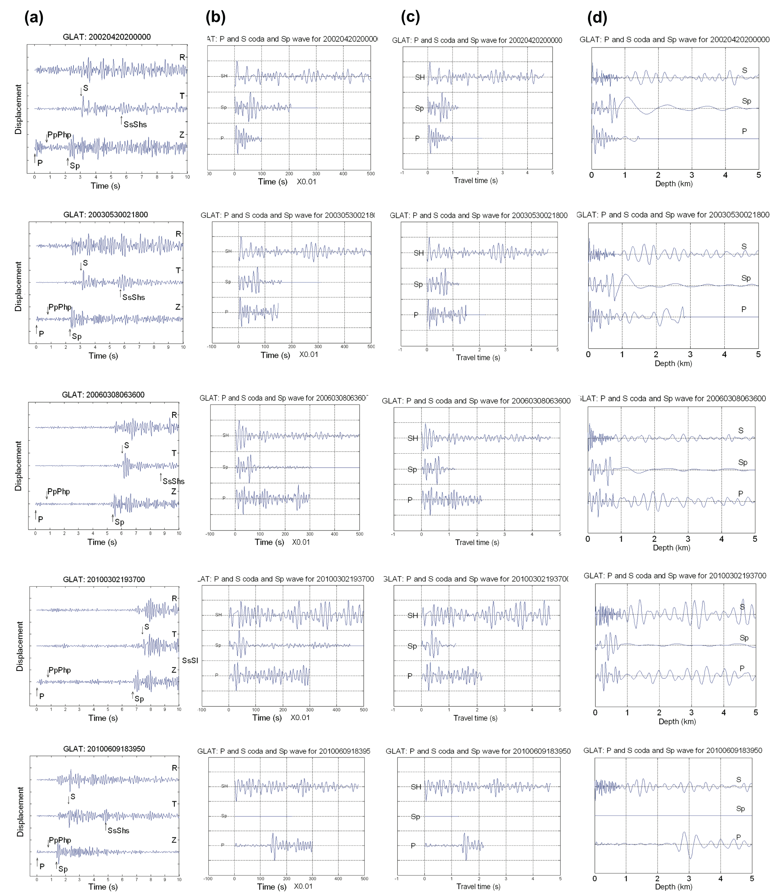
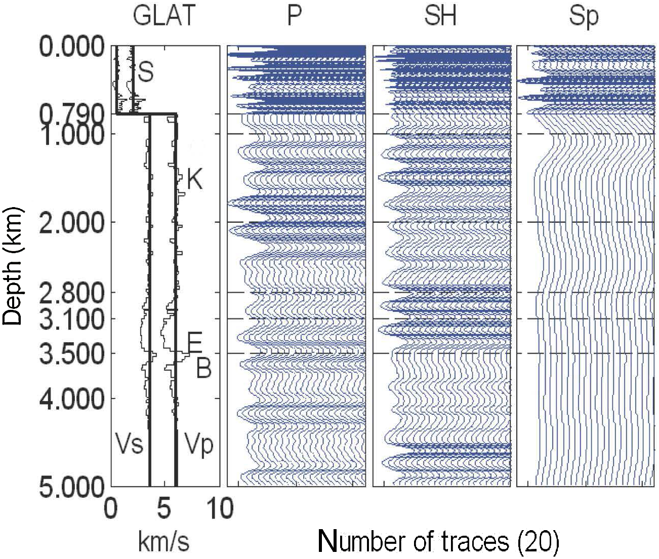
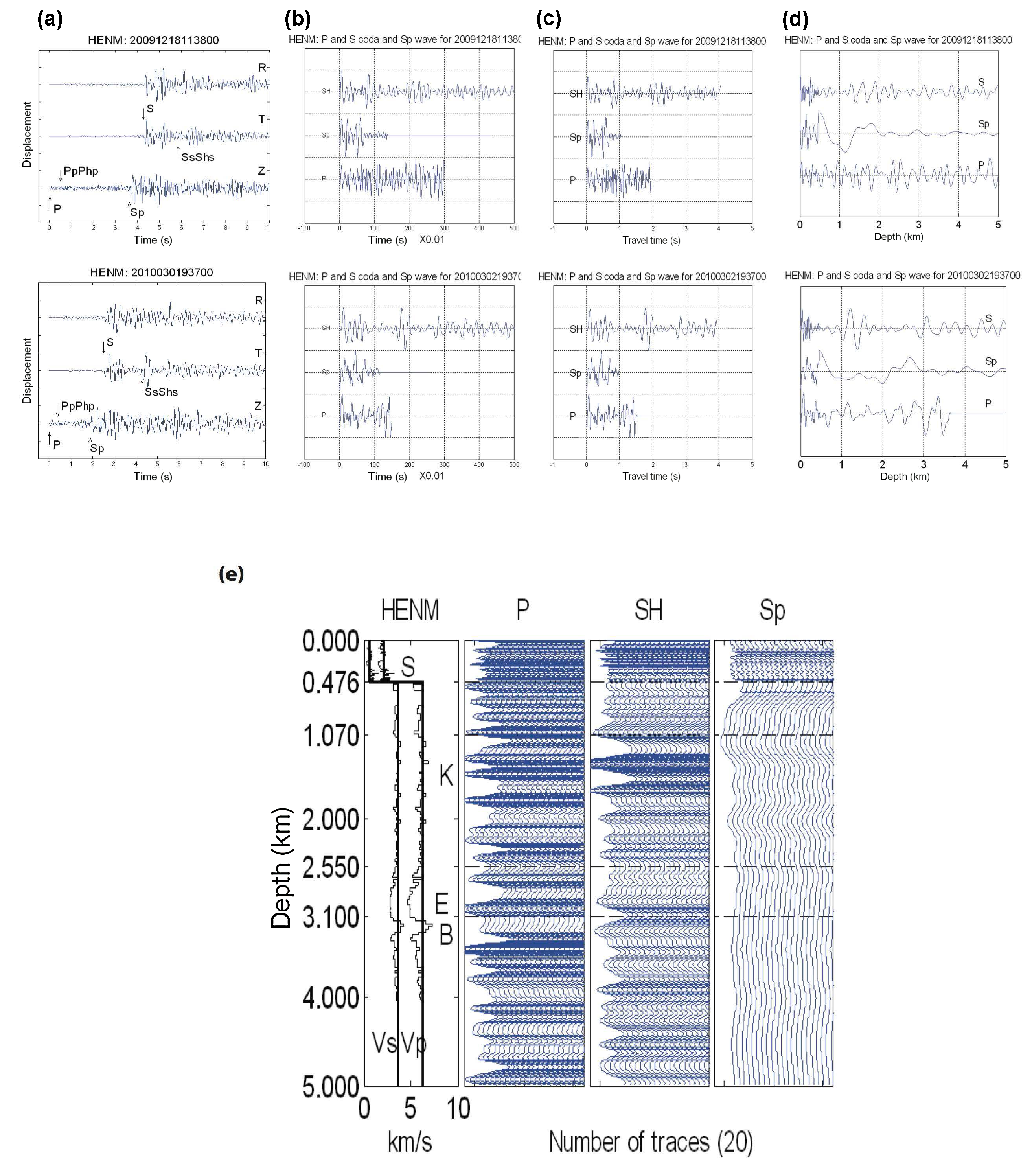
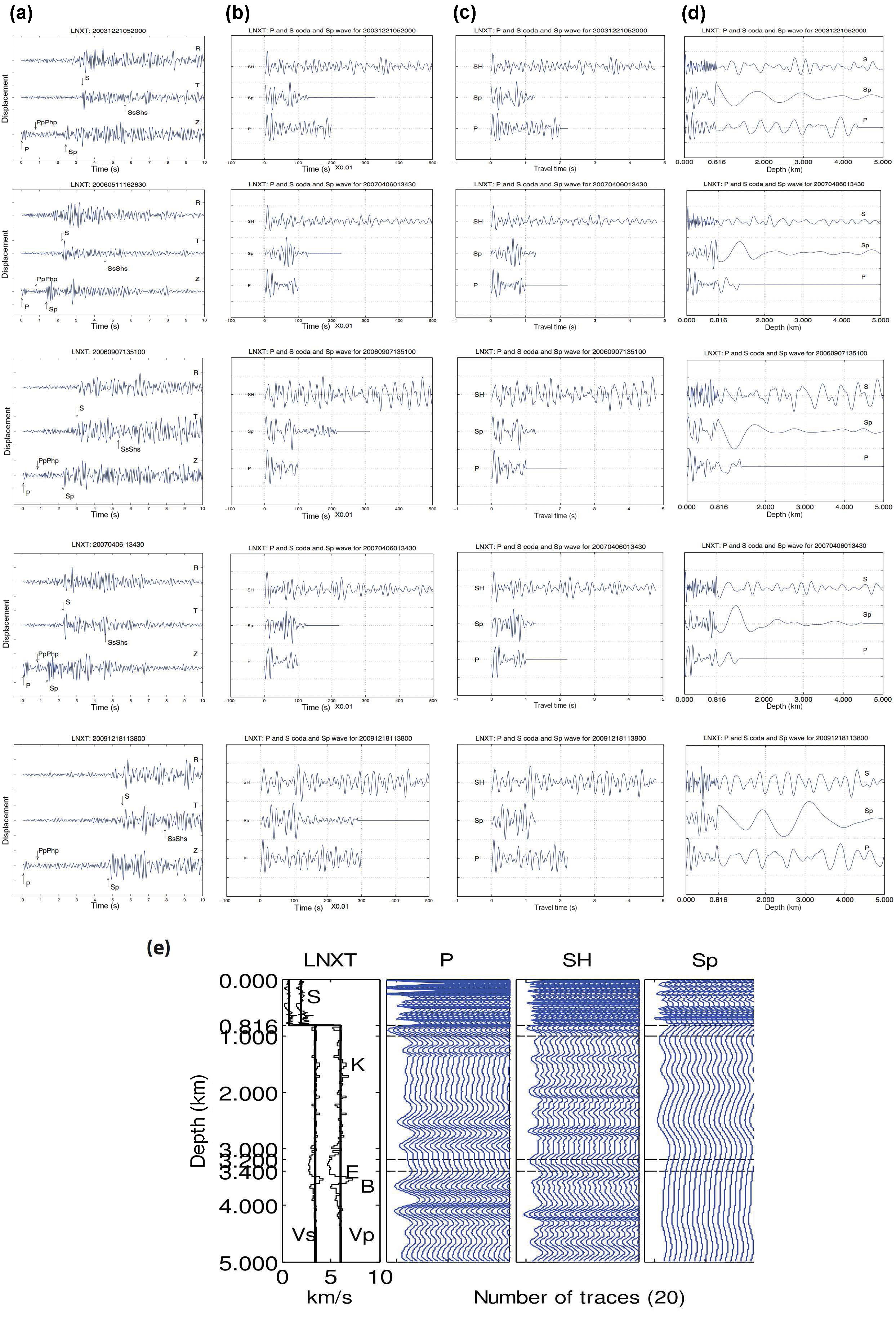
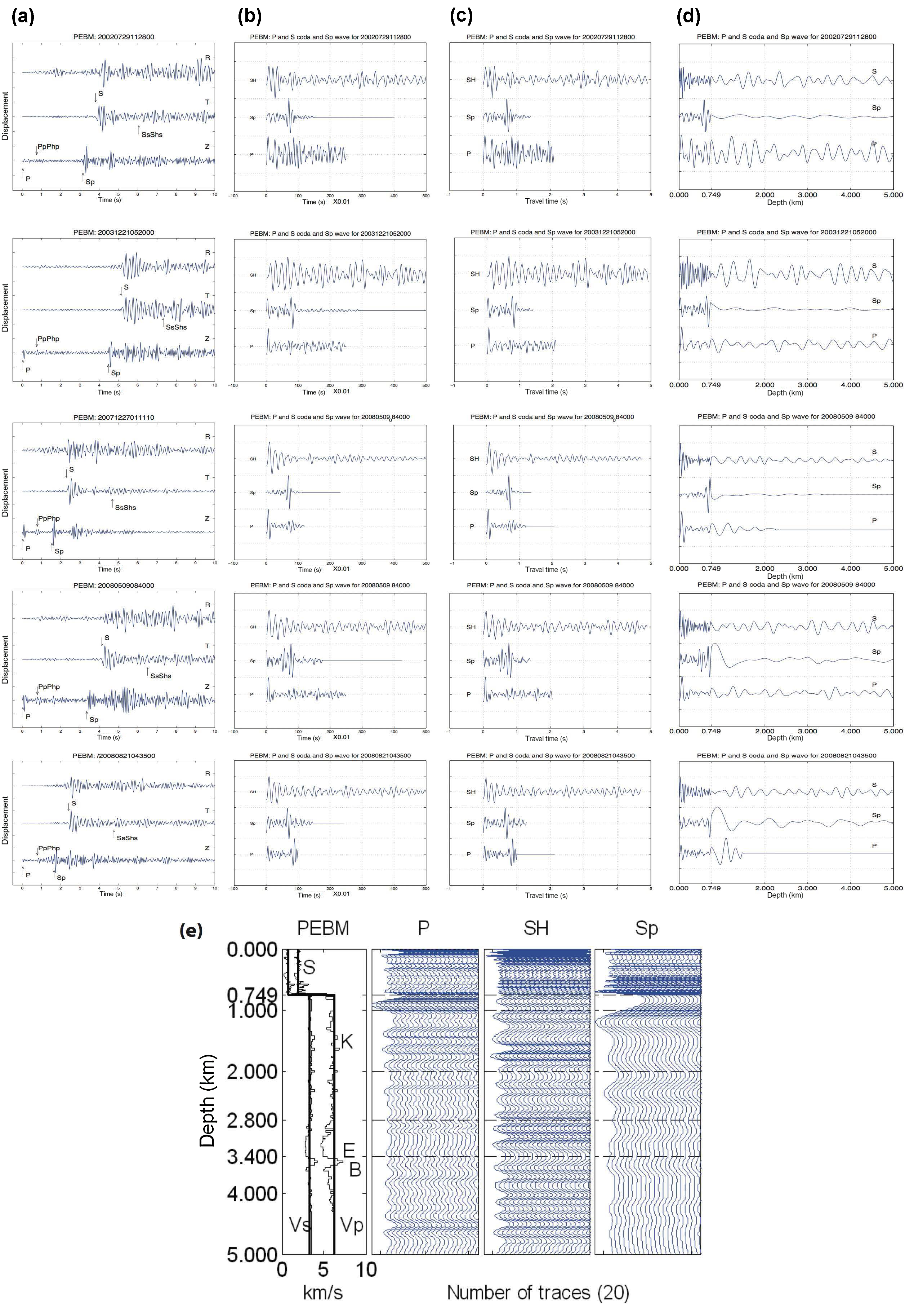
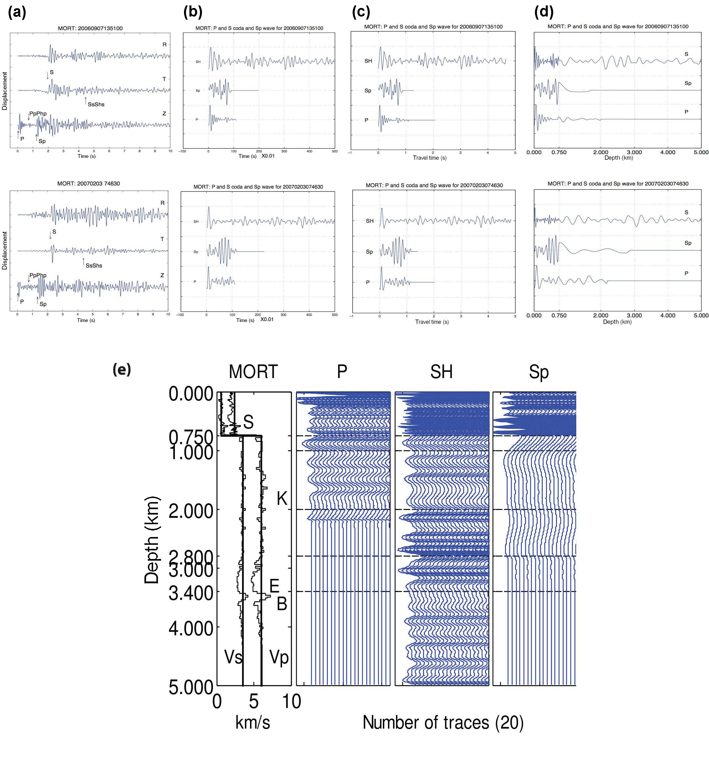
For Figures S3–S8, (a–d) are in the same format as in Figure S1: (a) earthquake displacement waveforms; (b) P, S, and time-reversed Sp waves in a function of time; (c) resampled P, S, and time-reversed Sp waves to a function of travel time; and (d) converted P, S, and time-reversed Sp waves to a function of depth.
For Figures S3–S8, (e) is in the same format as that in Figure S2.
Figure S1. GLAT pseudoprofiling: (a) Microearthquake displacement waveforms used in this study. Ground motion is sampled at 100 samples/s. P and S reflections and Sp phases are annotated. (b) P-wave coda ending before the Sp phase is taken from the Z component, and the S-wave coda is taken from the T component seismograms, both starting at the first peak of arrival. Sp waves are taken from the Z component seismograms in a time window after the P-wave coda to the peak of the SV-wave arrival at the R component and then are reversed in time. The first peak of the P- and S-wave coda and the Sp waves are placed as the zero reference time. A Butterworth causal band-pass filter is applied to the time series with corner frequencies of 0.5 and 5 Hz for P and Sp waves and of 0.5 and 10 Hz for the S wave such that all waves exhibit similar frequency waveforms. (c) Wave data are resampled to a function of two-way travel time for the P- and S-wave coda and one-way differential travel time for the Sp-wave to implement the normal moveout (NMO) corrections, extending to a depth of 5 km. (d) NMO-corrected P, S, and Sp waveforms are converted to a function of depth extended to 5 km. All waveforms are normalized to their individual maximum amplitude within the time or depth window for (a–d). Polarities of the peaks of the P, S, and Sp wave are corrected to downward motions.
Figure S2. GLAT pseudoprofiles: NMO-corrected and stacked pseudoprofiles constructed using a constant velocity layer of VP = 2.0 km/s and VS = 0.70 km/s overlying a half-space of VP = 6.0 km/s and VS = 3.5 km/s (thick lines). The detailed velocity model is included as thin lines. The depth scale in kilometers is the same on the y axis for all four panels. Amplitudes of all stacked traces beneath the sediments have been enlarged by a factor of 2 to enhance later arrivals in Paleozoic structure. The x axis is the number of repetitions of plotting the NMO-corrected stacked trace (20 times in this article). Dashed lines indicate common reflectors, and corresponding depths are labeled at the left of the figure. Strong reflectors correlate consistently to the interfaces at the boundary of the high-impedance contrast between sediments and Paleozoic rocks (0.790 km) and at the base of the Knox Group (2.8 km) and the Bonneterre Formation (3.5 km) in the deeper sedimentary structure. The pseudoprofilers imply that a low-velocity zone between the base of the Knox Group and the top of the Bonneterre Formation associates with the Elvins shale zone at depths of 2.8–3.5 km. A reflector at 1.0 km depth may associate with a dolomite layer. Interestingly, multiple SV-to-P conversions occur, beginning from the deeper interfaces. Representation of the stratigraphic strata is as follows: S, Mississippi Embayment Supergroup; K, Knox Group; E, Elvins shale; B, Bonneterre Formation marker.
Figure S3. GNAR pseudoprofiling: (a–d) are as described above, and (e) NMO-corrected and stacked pseudoprofiles computed using a constant velocity layer of VP = 2.0 km/s and VS = 0.65 km/s overlying a half-space of VP = 6.0 km/s and VS = 3.5 km/s. Strong reflectors appear to associate with the base of the supergroup at 0.762 km among all wave types, at depth 1 km, at the base of Knox Group at 2.95 km, and the Bonneterre Formation at 3.4 km between P and S waves.
Figure S4. HENM pseudoprofiling: (a–d) are as described above, and (e) NMO-corrected and stacked pseudoprofiles constructed using a constant velocity layer of VP = 2.1 km/s and VS = 0.65 km/s overlying a half-space of VP = 6.0 km/s and VS = 3.5 km/s. It reveals that strong reflectors can be associated with the base of the Mississippi Embayment Supergroup at depth 0.476 km, at the base of the Knox Group at 2.55 km, and the Bonneterre Formation at 3.1 km.
Figure S5. LNXT pseudoprofiling: (a–d) are as described above, and (e) NMO-corrected pseudoprofiles computed using a constant velocity layer of VP = 2.0 km/s and VS = 0.7 km/s overlying a half-space of VP = 6.0 km/s and VS = 3.4 km/s. It shows strong reflectors that can be associated with the Mississippi Embayment Supergroup at depth 0.816 km, at the base of the Knox Group at 3.0 km, and the high-velocity Bonneterre Formation marker at 3.4 km.
Figure S6. LPAR pseudoprofiling: (a–d) are as described above, and (e) NMO-corrected pseudoprofiles computed using a constant velocity layer of VP = 2.07 km/s and VS = 0.73 km/s overlying a half-space of VP = 6.1 km/s and VS = 3.5 km/s. It shows strong reflectors that can be associated with the Mississippi Embayment Supergroup at depth 0.855 km, the base of Knox Group at 3.0 km, and high-velocity Bonneterre Formation at 3.6 km.
Figure S7. PEBM pseudoprofiling: (a–d) are as described above, and (e) NMO-corrected pseudoprofiles computed using a constant velocity layer of VP = 1.95 km/s and VS = 0.70 km/s overlying a half-space of VP = 6.2 km/s and VS = 3.3 km/s. It shows a strong reflector that can be associated with the Mississippi Embayment Supergroup at 0.749 km depth among all wave types. Another two reflectors can be associated with the base of the Knox Group at 2.85 km and the high-velocity Bonneterre Formation at 3.4 km between P and S waves.
Figure S8. MORT pseudoprofiling: (a–d) are as described above, and (e) NMO-corrected pseudoprofiles computed using a constant velocity layer of VP = 2.42 km/s and VS = 0.62 km/s overlying a half-space of VP = 6.0 km/s and VS = 3.5 km/s. The imaging reveals a prominent reflector that can be associated with the Mississippi Embayment Supergroup at 0.750 km depth. It appears that there is a lack of rich frequency content in the short-period seismograms due to the narrow bandwidth in the instrumentation response. Apparently, there is not enough P-wave coda information to image the structure deeper than 2 km because separation time between P and S waves is shorter than 3 s.
[ Back ]