This electronic supplement contains tables of adjustment factors to convert selected ground-motion prediction equations (GMPEs) to the Swiss rock reference and figures showing trellis plots of all adjusted GMPEs with uncertainty estimates. Adjustment factors (CPSA,VS-κ0) are provided to convert selected GMPEs to the Swiss rock reference used in the probabilistic seismic-hazard analysis (PSHA), accounting for differences in the host rock VS profile and site attenuation (Tables S1–S4): Table S1 shows CPSA,VS-κ0 for the Akkar and Bommer (2010) model. Table S2 shows CPSA,VS-κ0 for the Cauzzi and Faccioli (2008) model. Table S3 shows CPSA,VS-κ0 for the Chiou and Youngs (2008) model. Table S4 shows CPSA,VS-κ0 for the Zhao et al. (2006) model.
Coefficients of the small magnitude adjustment (δ(M,R|T), equation 4 of the main article) are provided, along with values of δ(M,R|T) at various magnitude distance combinations for the Akkar and Bommer (2010) model (coefficients in Table S5, values in Table S6); the Cauzzi and Faccioli (2008) model (coefficients in Table S7, values in Table S8); the Chiou and Youngs (2008) model (coefficients in Table S9, values in Table S10); and the Zhao et al. (2006) model (coefficients in Table S11, values in Table S12).
Figures S1–S4 show trellis plots of all adjusted GMPEs (empirical and stochastic) used in the Swiss seismic-hazard maps. Figures S5–S7 show trellis plots of adjusted empirical GMPEs used in the Swiss seismic-hazard maps. Figures S8–S10 show trellis plots of the stochastic GMPEs for the Swiss alpine region used in the seismic-hazard maps. Figures S11–S13 show trellis plots of the stochastic GMPEs for the Swiss foreland region used in the seismic-hazard maps. Figures S14 and S15 show plots of the uncertainty models used in the Swiss seismic-hazard maps.
Figure S1. (Top left) Median values for peak ground acceleration (PGA), (top right) SA at T = 0.2 s, (lower left) SA at T = 1.0 s, and (lower right) SA at T = 2.0 s as estimated by empirical and stochastic GMPEs and plotted as functions of distance for a fixed moment magnitude (Mw 6).
Figure S2. (Top left) Median values for PGA, (top right) SA at T = 0.2 s, (lower left) SA at T = 1.0 s, and (lower right) SA at T = 2.0 s as estimated with empirical and stochastic GMPEs and plotted as functions of various moment magnitudes for a fixed Joyner–Boore distance (RJB = 10 km).
Figure S3. Median values of acceleration spectra SA estimated by empirical and stochastic GMPEs as functions of different moment magnitudes (from top to bottom) and short RJB distances (from left to right).
Figure S4. Median values of acceleration spectra SA estimated by empirical and stochastic GMPEs as functions of different moment magnitudes (from top to bottom) and long RJB distances (from left to right).
Figure S5. (Top left) Median values for PGA, (top right) SA at T = 0.2 s, (lower left) SA at T = 1.0 s, and (lower right) SA at T = 2.0 s as estimated by empirical GMPEs and plotted as functions of distance for a fixed moment magnitude (Mw 6).
Figure S6. (Top left) Median values for PGA, (top right) SA at T = 0.2 s, (lower left) SA at T = 1.0 s, and (lower right) SA at T = 2.0 s as estimated with empirical GMPEs and plotted as functions of various moment magnitudes for a fixed Joyner–Boore distance (RJB = 10 km).
Figure S7. Median values of SA estimated by empirical GMPEs as functions of different moment magnitudes (from top to bottom) and RJB distances (from left to right).
Figure S8. (Top left) Median values for PGA, (top right) SA at T = 0.2 s, (lower left) SA at T = 1.0 s, and (lower right) SA at T = 2.0 s as estimated by stochastic GMPEs (Swiss alpine) and plotted as functions of distance for a fixed moment magnitude (Mw 6).
Figure S9. (Top left) Median values for PGA, (top right) SA at T = 0.2 s, (lower left) SA at T = 1.0 s, and (lower right) SA at T = 2.0 s as estimated with stochastic GMPEs (Swiss alpine) and plotted as functions of various moment magnitudes for a fixed Joyner–Boore distance (RJB = 10 km).
Figure S10. Median values of SA estimated by stochastic GMPEs (Swiss alpine) as functions of different moment magnitudes (from top to bottom) and RJB distances (from left to right).
Figure S11. (Top left) Median values for PGA, (top right) SA at T = 0.2 s, (lower left) SA at T = 1.0 s, and (lower right) SA at T = 2.0 s estimated by stochastic GMPEs (Swiss Foreland) and plotted as functions of distance for a fixed moment magnitude (Mw 6).
Figure S12. (Top left) Median values for PGA, (top right) SA at T = 0.2 s, (lower left) SA at T = 1.0 s, and (lower right) SA at T = 2.0 s as estimated with stochastic GMPEs (Swiss Foreland) and plotted as functions of various moment magnitudes for a fixed Joyner–Boore distance (RJB = 10 km).
Figure S13. Median values of SA estimated by stochastic GMPEs (Swiss Foreland) as functions of different moment magnitudes (from top to bottom) and RJB distances (left to right).
Figure S14. Total and single-station sigma as a function of distance. Dashed lines represent original GMPE total sigmas, and solid and dashed-dotted lines represent implemented single-station sigma.
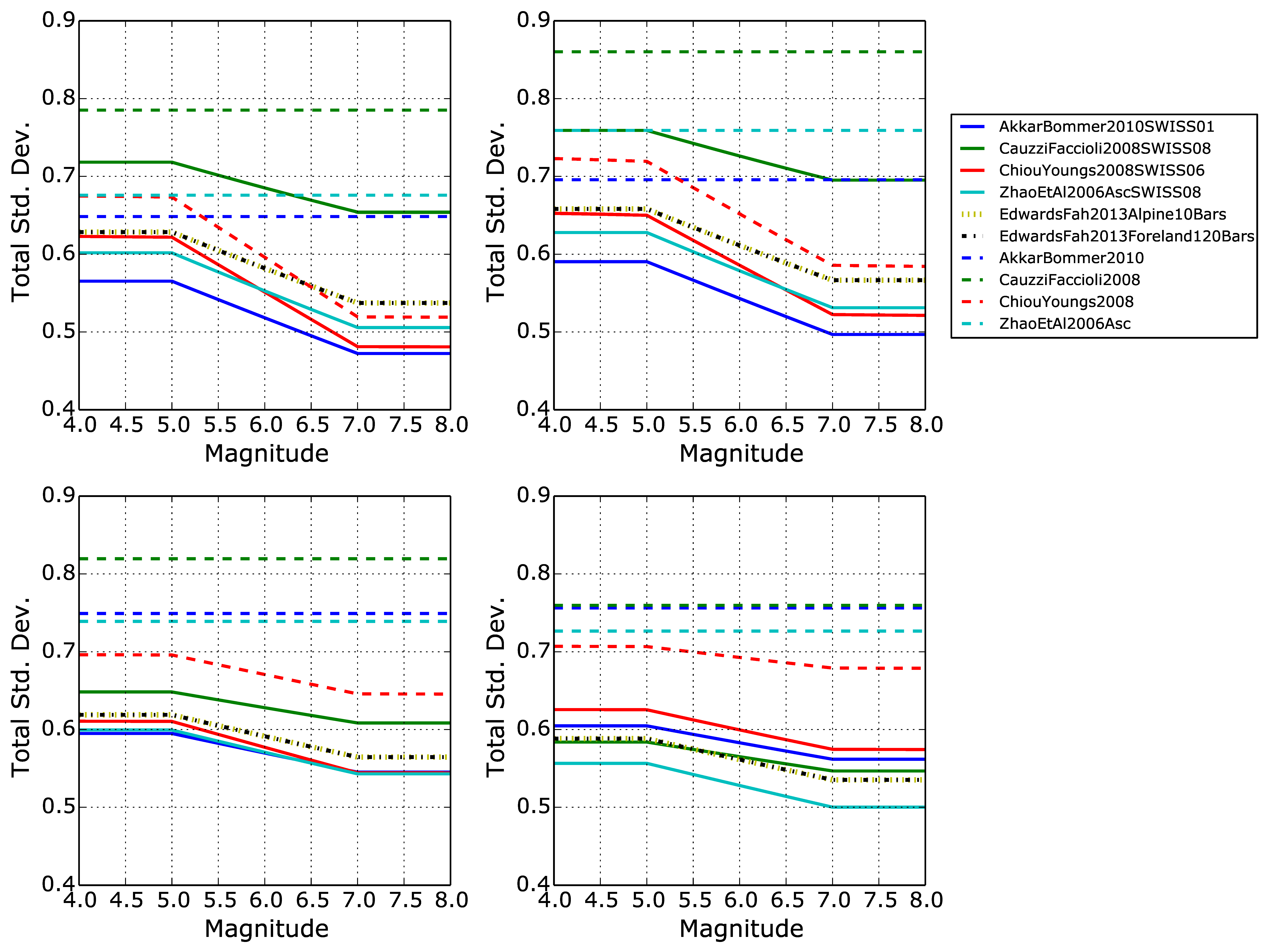
Figure S15. Total and single-station sigma as a function of magnitude. Dashed lines represent original GMPE total sigma, and solid and dashed-dotted lines represent implemented single-station sigma.
Table S1 [Plain Text Comma-separated Values; 7 KB]. CPSA,VS-κ0 for the Akkar and Bommer (2010) model. CPSA,VS-κ0 1–4 use the host VS profile form of Boore and Joyner (1997) with VS30 600 m/s. CPSA,VS-κ0 5–8 use the host VS profile form of Poggi et al. (2011) with VS30 600 m/s. CPSA,VS-κ0 1 and 5 use Δκ = 0.0061 s; CPSA,VS-κ0 2 and 6 use Δκ = 0.0091 s; CPSA,VS-κ0 3 and 7 use Δκ = 0.0136 s; and CPSA,VS-κ0 4 and 8 use Δκ = 0.0237 s.
Table S2 [Plain Text Comma-separated Values; 20 KB]. CPSA,VS-κ0 for the Cauzzi and Faccioli (2008) model. CPSA,VS-κ0 1–4 use the host VS profile form of Boore and Joyner (1997) with VS30 700 m/s. CPSA,VS-κ0 5–8 use the host VS profile form of Poggi et al. (2013) with VS30 700 m/s. CPSA,VS-κ0 1 and 5 use Δκ = 0.0048 s; CPSA,VS-κ0 2 and 6 use Δκ = 0.0063 s; CPSA,VS-κ0 3 and 7 use Δκ = 0.0064 s; and CPSA,VS-κ0 4 and 8 use Δκ = −0.0038 s.
Table S3 [Plain Text Comma-separated Values; 2 KB]. CPSA,VS-κ0 for the Chiou and Youngs (2008) model. CPSA,VS-κ0 1–4 use the host VS profile form of Boore and Joyner (1997) with VS30 620 m/s. CPSA,VS-κ0 5–8 use the host VS profile form of Poggi et al. (2011) with VS30 620 m/s. CPSA,VS-κ0 1 and 5 use Δκ = 0.0059 s; CPSA,VS-κ0 2 and 6 use Δκ = 0.0085 s; CPSA,VS-κ0 3 and 7 use Δκ = 0.0105 s; and CPSA,VS-κ0 4 and 8 use Δκ = 0.0206 s.
Table S4 [Plain Text Comma-separated Values; 2 KB]. CPSA,VS-κ0 for the Zhao et al. (2006) model. CPSA,VS-κ0 1–4 use the host VS profile form of Boore and Joyner (1997) with VS30 700 m/s. CPSA,VS-κ0 5–8 use the host VS profile form of Poggi et al. (2013) with VS30 700 m/s. CPSA,VS-κ0 1 and 5 use Δκ = 0.0048 s; CPSA,VS-κ0 2 and 6 use Δκ = 0.0064 s; CPSA,VS-κ0 3 and 7 use Δκ = 0.0093 s; and CPSA,VS-κ0 4 and 8 use Δκ = 0.0194 s.
Table S5 [Plain Text Comma-separated Values; 5 KB]. Coefficients of the small magnitude adjustment (δ(M,R|T), equation 4 of the main article) for the Akkar and Bommer (2010) model. #N/A indicates no coefficient was computed for this period; Log–linear interpolation was used between the lower and upper bounding coefficients at this period.
Table S6 [Plain Text Comma-separated Values; 23 KB]. Tabulated values of the small magnitude adjustment (δ(M,R|T)) for various magnitude–distance combinations are provided for the Akkar and Bommer (2010) model.
Table S7 [Plain Text Comma-separated Values; 17 KB]. Coefficients of small magnitude adjustment (δ(M,R|T), equation 4 of the main article) for the Cauzzi and Faccioli (2008) model.
Table S8 [Plain Text Comma-separated Values; 65 KB]. Tabulated values of the small magnitude adjustment (δ(M,R|T)) for various magnitude–distance combinations are provided for the Cauzzi and Faccioli (2008) model.
Table S9 [Plain Text Comma-separated Values; 2 KB]. Coefficients of small magnitude adjustment (δ(M,R|T), equation 4 of the main article) for the Chiou and Youngs (2008) model.
Table S10 [Plain Text Comma-separated Values; 9 KB]. Tabulated values of the small magnitude adjustment (δ(M,R|T)) for various magnitude–distance combinations are provided for the Chiou and Youngs (2008) model.
Table S11 [Plain Text Comma-separated Values; 2 KB]. Coefficients of small magnitude adjustment (δ(M,R|T), equation 4 of the main article) for the Zhao et al. (2006) model.
Table S12 [Plain Text Comma-separated Values; 9 KB]. Tabulated values of the small magnitude adjustment (δ(M,R|T)) for various magnitude–distance combinations are provided for the Zhao et al. (2006) model.
Akkar, S., and J. J. Bommer (2010). Empirical equations for the prediction of PGA, PGV, and spectral accelerations in Europe, the Mediterranean region, and the Middle East, Seismol. Res. Lett. 81, 195–206.
Boore, D. M., and W. B. Joyner (1997). Site amplifications for generic rock sites, Bull. Seismol. Soc. Am. 87, 327–341.
Cauzzi, C., and E. Faccioli (2008). Broadband (0.05 to 20 s) prediction of displacement response spectra based on worldwide digital records, J. Seismol. 12, 453–475.
Chiou, B. S. J., and R. R. Youngs (2008). An NGA model for the average horizontal component of peak ground motion and response spectra, Earthq. Spectra 24, 173–215.
Poggi, V., B. Edwards, and D. Fäh (2011). Derivation of a reference shear-wave velocity model from empirical site amplification, Bull. Seismol. Soc. Am. 101, 258–274.
Poggi, V., B. Edwards, and D. Fäh (2013). Reference S-wave velocity profile and attenuation models for ground-motion prediction equations: Application to Japan, Bull. Seismol. Soc. Am. 103, 2645–2656.
Zhao, J. X., J. Zhang, A. Asano, Y. Ohno, T. Oouchi, T. Takahashi, H. Ogawa, K. Irikura, H. K. Thio, P. G. Somerville, et al. (2006). Attenuation relations of strong ground motion in Japan using site classification based on predominant period, Bull. Seismol. Soc. Am. 96, 898–913.
[ Back ]