This electronic supplement develops several theoretical and practical aspects of implementing the correlation and cone detector on geophysical waveform data. The Effective Degrees of Freedom section documents an estimator for the number of statistically independent samples NE in a data stream and describes how it shapes the correlation statistic’s probability density function (PDF). In The Maximum-Likelihood Correlation Statistic section, we derive this PDF, which quantifies our correlation and cone detector’s ability to identify their respective target waveforms. The Cone Detector Statistic section then presents an alternative to the correlation detector hypothesis test and introduces additional, deterministic uncertainty into the target signal model. Therein, we derive the cone detector PDF, illustrate its geometric properties, and model its capability to detect template-decorrelated target waveforms. We support this derivation with Monte Carlo simulations (Fig. S1) and illustrate how deterministic template-target waveform decorrelation inflates thresholds relative to the correlation case (Fig. S2). The Relative Magnitude Parameterization of the Cone Detector Statistic section then relates the probability of detecting a template-decorrelated target waveform to the magnitude of the seismic source that produces this target waveform. Finally, we provide an analysis of three ostensible sources of error from our data processing implementation in the Error Analyses section and describe their influence on our threshold and capability analyses. We find that only data-variance pooling is likely to appreciably affect detector performance.
This section outlines a method to estimate the effective degrees of freedom NE of a data stream x as . This estimate provides an ostensible alternative to a full covariance matrix for x that is generally required for temporally or spatially correlated data. Density functions for detection statistics that process x are then easily parameterized by the effective number of independent data-stream samples NE. This scalar theoretically equates to twice the time (T) bandwidth (B) product (2TB) of the data stream over the temporal duration of the correlation template. Real data often show that , however. This occurs both naturally and through processing operations like band-pass filtering, which replace each sample with itself plus a weighted sum of its neighbors and thereby introduce intersample statistical dependence. To quantify the influence such correlation exerts on the shape of our detector’s PDF curves, we implement an empirical estimator for NE, denoted , to continuously update such PDF parameterizations (e.g., the correlation statistic PDF ). This estimator computes the sample correlation between the multichannel template waveform w and several hundred pseudorandom, commensurate data vectors drawn from nonintersecting segments of preprocessed, signal sparse data within x (see Weichecki-Vergara et al., 2001, their section 2.4). We compute the sample variance of the resultant correlation time series using 99.9% of the data by excluding 0.01% of the extreme left and right tails of its histogram. This provides the needed statistic to estimate NE as
(S1)
We use to parameterize (equation S7), compute detector thresholds , and quantify detector performance.
This section develops the PDF and detection performance of the sample correlation detection statistic r(x) (equation 3 of the main article). Because the form of the sample correlation PDF differs from that reported elsewhere, we derive the general form here.
The relative square error in approximating a data stream (the model of equation 15 of the main article), with a waveform template w, is the ratio of the least-squares error to measured signal energy . This error may be rewritten as a ratio of quadratic forms
(S2)
in which is the maximum-likelihood estimate (MLE) for template waveform amplitude. We now rewrite the right side of the second equality in equation (S2) as a ratio of subspace projections
(S3)
in which W is the subspace span (w), is the orthogonal complement to W, PW is the projector onto W, and is the projector onto . The denominator follows from the Pythagorean identity for Hilbert spaces. We define two noncentrality parameters from these terms
(S4)
in which the expected value and linear-projection operators commute. We combine the previous three equations to rewrite r2(x)
(S5)
in which is distributional equality, is the noncentral chi-square distribution with NE −1 degrees of freedom and noncentrality parameter , and is the noncentral chi-square distribution with one degree of freedom and noncentrality parameter . From the definition of the beta distribution
(S6)
(Kay, 1998), in which is the doubly noncentral beta distribution function. It is evaluated at (with the same domain as r2), has N1 and N2 degrees of freedom and noncentrality parameters and . The presence or absence of a target signal is indexed by the hypothesis on the data. Hypothesis symbolizes that the data consist of only noise, whereas signifies that the data consist of a signal plus noise. The scalar NE denotes the effective number of independent samples within x. When the data stream contains only noise, the hypothesis is satisfied, and r2 has a central beta distribution, in which . In the presence of signal, the data stream x generally has nonzero projections and that are respectively onto and orthogonal to the noise-contaminated template data vector w. In this case, , , and r2 has doubly noncentral beta distribution. If the target signal is an amplitude-scaled copy of the template waveform, then , , and r2 has a noncentral beta distribution. The singly noncentral beta distribution therefore provides an absolute upper bound on the detection performance of a correlation detector consistent with assumptions underlying .
We derive the PDF for from the density of r2 using a variable transformation; we additionally consider values r < 0, so that
(S7)
The form of this distribution function differs from that derived in similar applications (Weichecki-Vergara et al., 2001). In the alternative case, the signal-present data stream was assumed to correlate sample-by-sample with the template waveform, and the test statistic had a Pearson moment-product distribution.
This section develops the cone detection statistic (equation 17 of the main article), its PDF, and illustrates its performance; it was originally introduced in the context of icequake detection (Carmichael, 2013). We first reference the two competing hypotheses of equation (15) of the main article
(S8)
We further assume that preprocessing operations (like filtering) and naturally occuring temporal data correlation reduces the number of statistically independent samples in x to . Given this parameterization, the PDF under is denoted as and the PDF under as , in which
(S9)
We estimate the unknown parameters under each model listed in equation (15) of the main article and select the applicable hypothesis using a log-generalized likelihood ratio test (log-GLRT). This test evaluates the PDFs for the competing hypotheses at the MLEs of their unknown parameter values and then compares their log ratio to a threshold value . The test’s decision rule is a conditional, scalar inequality
(S10)
The MLE of the variance under each hypothesis is
(S11)
(Kay, 1993; Scharf and Friedlander, 1994), in which the subscripts on each sample variance estimate in equation (S11) indicate the applicable hypothesis, and N is the number of samples in x, not to be confused with NE. To estimate the distribution mean under , we evaluate at the MLE for and perform a constrained maximization of
(S12)
The solution to this equation
(S13)
is the MLE for u. That is, is the vector that minimizes the distance between the observed data x and all points that constitute the multiplet set . This defines the projection of x onto as the unique signal that is either interior to, or on the boundary of (Stark and Yang, 1998). The sample variance and cone-element MLEs from equation (S11) reduce to
(S14)
We obtained equation (S14) without specifying aside from its convexity. This result therefore applies to any normally distributed data confined in a convex set. In the case that is described by the correlation constraint of equation (14) of the main article, the projection energy has a conic decomposition
(S15)
as given by Moreau’s decomposition theorem (Moreau, 1962), which is analogous to the orthogonal subspace decomposition from linear analysis (Stark and Yang, 1998). The log ratio is then expressible as
(S16)
The right side of equation (S14) is of the form , which is monotonically increasing for . Because , equation (S16) may be inverted for its argument to provide an equivalent test statistic s(x) for the decision rule introduced in equation (S10)
(S17)
Equation (S17) demonstrates that s(x) compares the ratio of the projected signal energy to the original signal energy. The exact projection of x, from a general Hilbert space and onto , is derived in Stark and Yang (1998, pp. 111–113). Vector is a nonlinear projection that depends on the value of x and is either in , on its boundary , or zero. We document an equivalent form of that projection here
(S18)
The constants and vectors in equation (S18) are
(S19)
The vector in equation (S19) is the normalized multichannel template waveform defined by equation (14) of the main article, not to be confused with a parameter estimate. Using the definitions in equation (S19), the test statistic s(x) of equation (16) of the main article is then expressible as
(S20)
The detection statistic s(x) must be equivalent to the correlation coefficient as approaches a limiting value of 1. To demonstrate this, we first note that any projected signal has a decreasing probability of lying inside the cone as decreases (equation S20). Similarly, any projected signal has a decreasing probability zero of lying on the cone vertex. It follows that only the projection onto the limiting cone boundary is nontrivial, so that
(S21)
in which is the limit of approaching from values less than 1, whereby .
We derive the requisite PDF for s(x) from its cumulative distribution function (CDF) using the law of total probability. In words, this law states that the probability that the cone statistic random variable S takes on a value as large as s(x) is the sum of three conditional probabilities: the probability that (1) , given , plus (2) the probability , given , plus (3) the probability that , given
(S22)
in which is the conditional probability of A, given B is true and statement is equivalent to . To express in a computationally evaluable form, we write its three conditioning factors in terms of through equation (S20). Two of these terms are trivial to evaluate from the definition for
(S23)
The other terms in equation (S22) are expressible using through equation (S20)
(S24)
We evaluate these probabilities by developing the CDF for the ratio (). To do so, we make a change of variables with
(S25)
in which is the CDF for correlation statistic . We then use equation (S25) to write the identities from equation (S24) in terms of :
(S26)
Last, we evaluate the derivative of in equation (S22) through a variable change on , in which . To do so, we first note that is invertible over this domain and express r as a function of s
(S27)
The PDF of s(x) over is therefore
(S28)
in which indicates the restricted domain of . To obtain the PDF for s(x) over , we differentiate equation (S22) and substitute equations (S26) and (S28) into the results. This produces a density function that depends on only s, c, and
(S29)
because the top line of equation (S22) is constant and differentiates to zero.
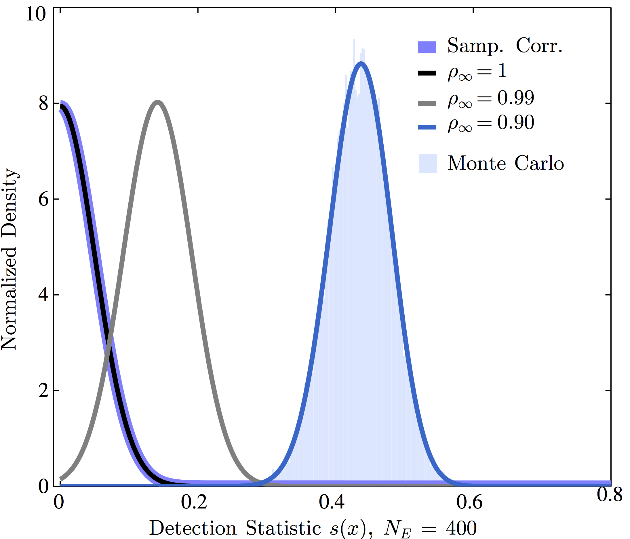
We assessed the validity of our derivation using a Monte Carlo simulation, whereby we projected random noise and noise-contaminated signal vectors onto several convex cones of increasing aperture and computed the statistic s(x). This simulation demonstrates that equation (S29) agrees with our empirical histograms (Fig. S1).
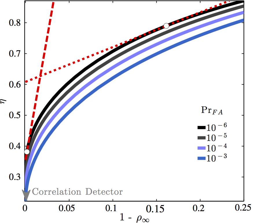
We additionally compared our cone detector thresholds against constant false-alarm-on-noise constraints. We thereby inverted for cone detector thresholds using a fixed value for the effective degrees of freedom () over a grid of decorrelation parameters () that ranged from 0 to 0.25. We repeated this process for several false alarm rates (Fig. S2). The resulting detection thresholds increase most rapidly for small changes near , at which the signal space of the cone geometrically collapses to the 1D subspace used by the associated correlation detector. The slope of the curves here may become undefined. We will explore this result more quantitatively in future work.
An unbiased estimator for the relative magnitude between an explosion that generates a noisy waveform and an explosion that generates a detector template w is
(S30)
(Carmichael and Hartse, 2016, their equation B.8), in which denotes an estimate for noise variance in x (subscript denotes hypothesis is true) and N is the number of samples in x, not to be confused with NE. To relate to the noncentrality parameters and that shape the PDF , we again use the standard Pythagorean identity for Hilbert spaces
(S31)
in which the subspace projection terms are defined in equation (S3). Next, we use the definitions of u, , and to rewrite as
(S32)
in which “noise term” is an inner product expression that includes n, and is the true variance of the target data. The noncentrality parameters in equation (S32) are related by Carmichael and Hartse (2016, their equation A.11)
(S33)
and the expected value of “noise term” in equation (S32) is
(S34)
in which , because the noise is zero mean. Finally, we combine the preceding equations (this section), remove the noise-bias term , and write in terms of relative magnitude
(S35)
Equation (S35) thereby expresses the noncentrality parameter for both the correlation and cone detection statistic in terms of the four fundamental scalars describing the wavefield: the deterministic correlation between the template and target waveforms, the signal energy of the template waveform, the noise variance of the target data, and the relative magnitude between the template and target source.
For our purposes, equation (S35) parameterizes by relative magnitude. In such cases, the term is estimable from equation (12) of the main article, is estimable from the top term of equation (S11), and is effectively deterministic because correlation detectors generally implement high-signal-to-noise ratio (SNR) templates.
We identified three potentially significant sources (risks) of error in our detection capability assessments and empirical comparison. The first risk of error is attributable to certain details of template selection. Specifically, waveforms recorded on International Monitoring System (IMS) arrays with large differences in source–receiver separation distance show temporal gaps in start time of the high-SNR portions of the recorded signals and therefore require sample imputation. Zero padding such data to equalize length can lead to several biases, however. For example, supplementing data with a large number of zeros causes the empirical null PDF (histogram) for the correlation detection statistic to become more concentrated around its mean and thereby artificially lowers the detector’s threshold. The statistic histogram then fits the predicted PDF poorly and biases estimates of the degree of freedom parameter , because the correlation variance is reduced by the presence of zeros (equation S1). To mitigate these problems and facilitate template scanning, we therefore abstained from zero-padding the intermediate, noisy portion of our waveform template. Instead, we shifted each seismogram channel by an amount equal to its start time, minus the earliest start time among all template channels (template and target data). We thereby maintained the signal-only length of our template, avoided padding, and kept all data aligned to the same origin time. In addition to preventing estimation bias, this shifting mitigated needless computation of padded data and prevented divide-by-zero errors. We therefore consider our template selection to present a low (direct) risk of error.
Estimation of presents a second potential source of error. This arises largely from ambiguous estimation schemes for waveform SNR, which influence the variability of (equation 11 of the main article), which, in turn, inversely scales (equation 12 of the main article). We mitigated ambiguity problems by carefully selecting an associated low-variance estimate for SNR, which normalizes . One “common-sense” estimate for SNR is the ratio of an N-point sample variance estimate of the data proceeding the detected signal, divided by an N-point sample variance estimate of data preceding the detected signal (a renormalized short-term average/long-term average [STA/LTA]). It is obvious, however, that any such estimate will be biased by background signals contaminating the data steam, which reduce the resultant SNR estimate for u. It follows that will be a biased estimator and give lower-than-true deterministic correlation values. A better approach requires preprocessing target data with a power (STA/LTA) detector, removing samples that exceed a threshold for signal declaration, and then computing the noise variance from this remaining data. The quotient
(S36)
then gives a reduced-bias SNR estimate. We used this estimator to compute as:
(S37)
We therefore consider our estimates of to be robust and unlikely to induce significant uncertainty.
Last, noise variance estimation presents an additional risk of error. As we noted before (see the Estimating Deterministic Decorrelation section in the main article), background seismicity adds signal to the time series and can thereby bias such estimates. We therefore processed our target data in parallel with an STA/LTA detector that operated at a false-alarm-on-noise probability, removed data that exceeded the associated threshold, and used the remaining (almost) signal-free data to estimate noise variance on each IMS channel. This scheme thereby avoided bias from signal. A second form of bias was also present, however. This latter bias originated from the nonuniform number of channel samples processed by the detector. Specifically, we noted above that our template included large temporal gaps over portions of the waveform, and consequently, records from MJAR contribute less to each detection statistic than do longer duration records at MKAR. An alternative noise-variance estimate that accounts for such disparate channel contribution employs the pooled variance , given by
(S38)
in which is the noise-variance estimate from channel . We performed a subsequent analysis using this estimator and found that it was often smaller than our naive estimation that used equally weighted data. This would have increased the effective size of the noncentrality parameter that controls predicted detection power. It may explain why, at times, our observed detection capability exceeded the concurrent predicted detection capability. We therefore suggest that performance discrepancy may generally result from an inconsistency in noise variance estimation.
Figure S1. Null hypothesis PDFs for three cases of deterministic template-target waveform correlation uncertainty: , , (in which NE = 400). The PDFs for r(x) and s(x) equate for identically shaped waveforms as shown by the purple and black curves. The shaded region shows a Monte Carlo simulation of the PDF for s(x) when
Figure S2. Cone detector thresholds (equation 21 of the main article) for constant values of compared against deterministic uncertainty in the template-target waveform cross correlation , in which . The leftmost tangent line to the curve shows a rapid increase in for small uncertainties in deterministic template-to-target waveform correlation relative to near-linear increases in for larger uncertainties. corresponds to the correlation detector.
Carmichael, J. D. (2013). Melt-triggered seismic response in hydraulically-active polar ice: Observations and methods, Ph.D. Thesis, University of Washington, Seattle, Washington.
Carmichael, J. D., and H. Hartse (2016). Threshold magnitudes for a multichannel correlation detector in background seismicity, Bull. Seismol. Soc. Am. 106, no. 2, 478–498.
Kay, S. M. (1993). Fundamentals of Statistical Signal Processing: Estimation Theory, Prentice-Hall PTR, Englewood Cliffs, New Jersey.
Kay, S. M. (1998). Fundamentals of Statistical Signal Processing: Detection Theory, First Ed., Prentice-Hall Inc., Upper Saddle River, New Jersey.
Moreau, J.-J. (1962). Décomposition orthogonale dun espace hilbertien selon deux cônes mutuellement polaires, C.R. Acad. Sci. Paris 255, 238–240 (in French).
Scharf, L. L., and B. Friedlander (1994). Matched subspace detectors, IEEE Trans. Signal Process. 42, no. 8, 2146–2156.
Stark, H., and Y. Yang (1998). Vector Space Projections: A Numerical Approach to Signal and Image Processing, Neural Nets, and Optics, Wiley John and Sons, Incorporated, New York, New York.
Weichecki-Vergara, S., H. L. Gray, and W. A. Woodward (2001). Statistical development in support of CTBT monitoring, Technical Rept. DTRA-TR-00-22, Southern Methodist University.
[ Back ]