This electronic supplement contains details of processing procedure, figures of the empirical regional attenuation functional, and source terms of 1191 events from the Alto Tiberina fault (ATF) data set and earthquake catalog.
We briefly review the procedure used in this study, because more details of the data processing may be found in Malagnini and Dreger (2016). Each time history in our data set was corrected for the instrument response and visually examined to eliminate multiple events and spurious transient signals. Before handpicking P- and S-wave arrivals, at the operator’s discretion, overly noisy recordings were removed altogether. The selected traces were then band-pass filtered around a set of central frequencies, fi, using an eight-pole Butterworth high-pass filter with corner at , followed by an eight-pole low-pass filter with corner at .
After the described preprocessing, the observed time-domain peak spectra of the filtered time histories (indicated in what follows as ) were cast into the matrix form
(S1)
is the logarithm of the peak amplitude (kth station, jth event) observed on a narrow band-pass-filtered version of the nth time history. is the contribution of the jth source to an arbitrary hypocentral distance r0 = 15 km. represents the kth site term. indicates the propagation term, intended as the contribution of the crustal wave propagation that is common to all the recording sites.
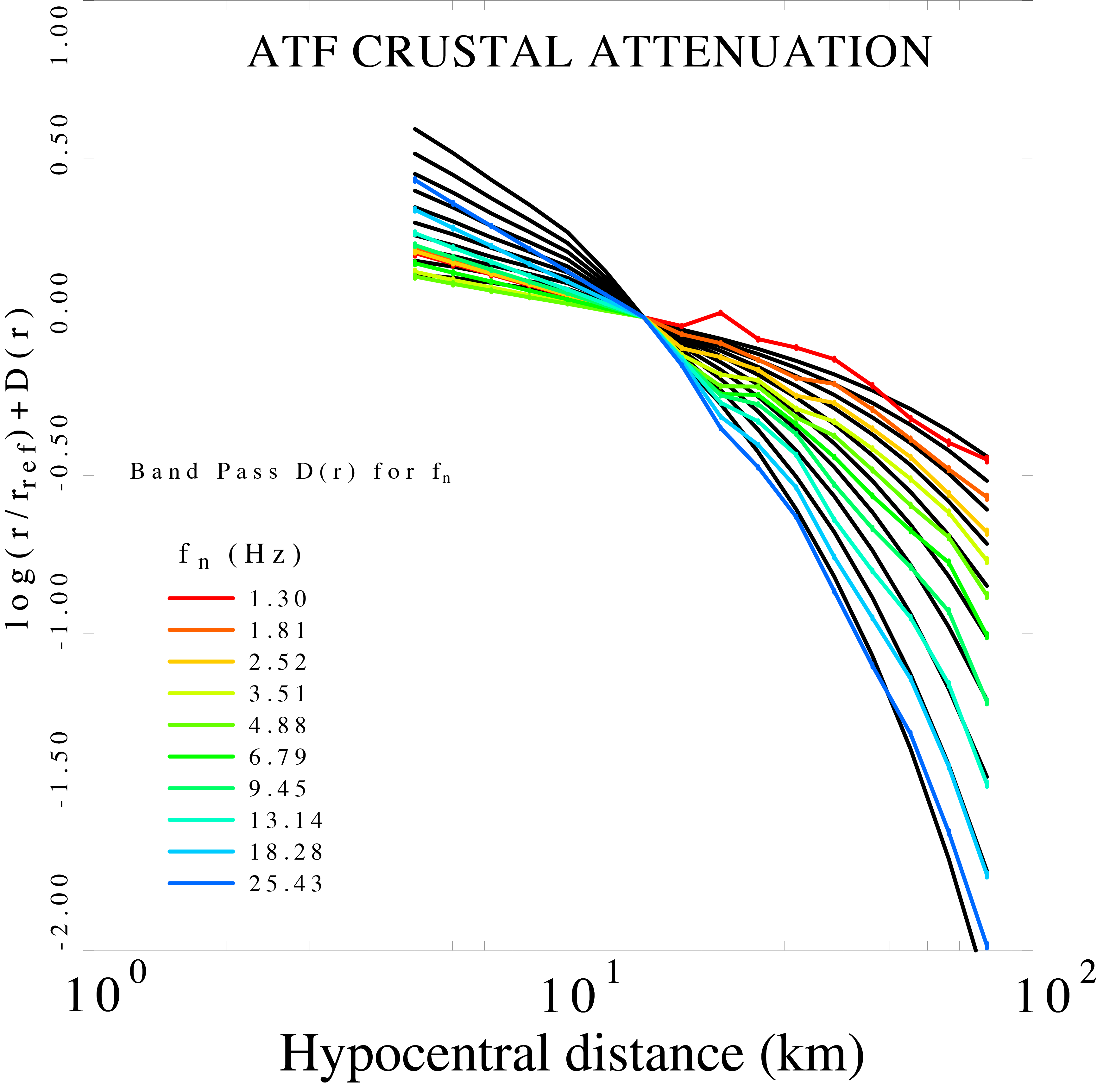
The regional attenuation term obtained for the area surrounding the ATF is shown in Figure S1. We modeled the empirical estimates of the peak amplitudes, as a function of hypocentral distance, at different sampling frequencies. Colored curves represent deviations from the 1/r trend for the normalized attenuation functions. Black curves in the background represent our theoretical predictions of the attenuation functions obtained for each central frequency with the following equation:
(S2)
The crustal attenuation is described as a combination of the effects of the geometrical spreading g(r) and of the anelastic attenuation represented by the quality factor Q(f). The best fit is obtained with the following values, in which (fref= 1.0 Hz), and the geometrical spreading function at all distances are
(S3)
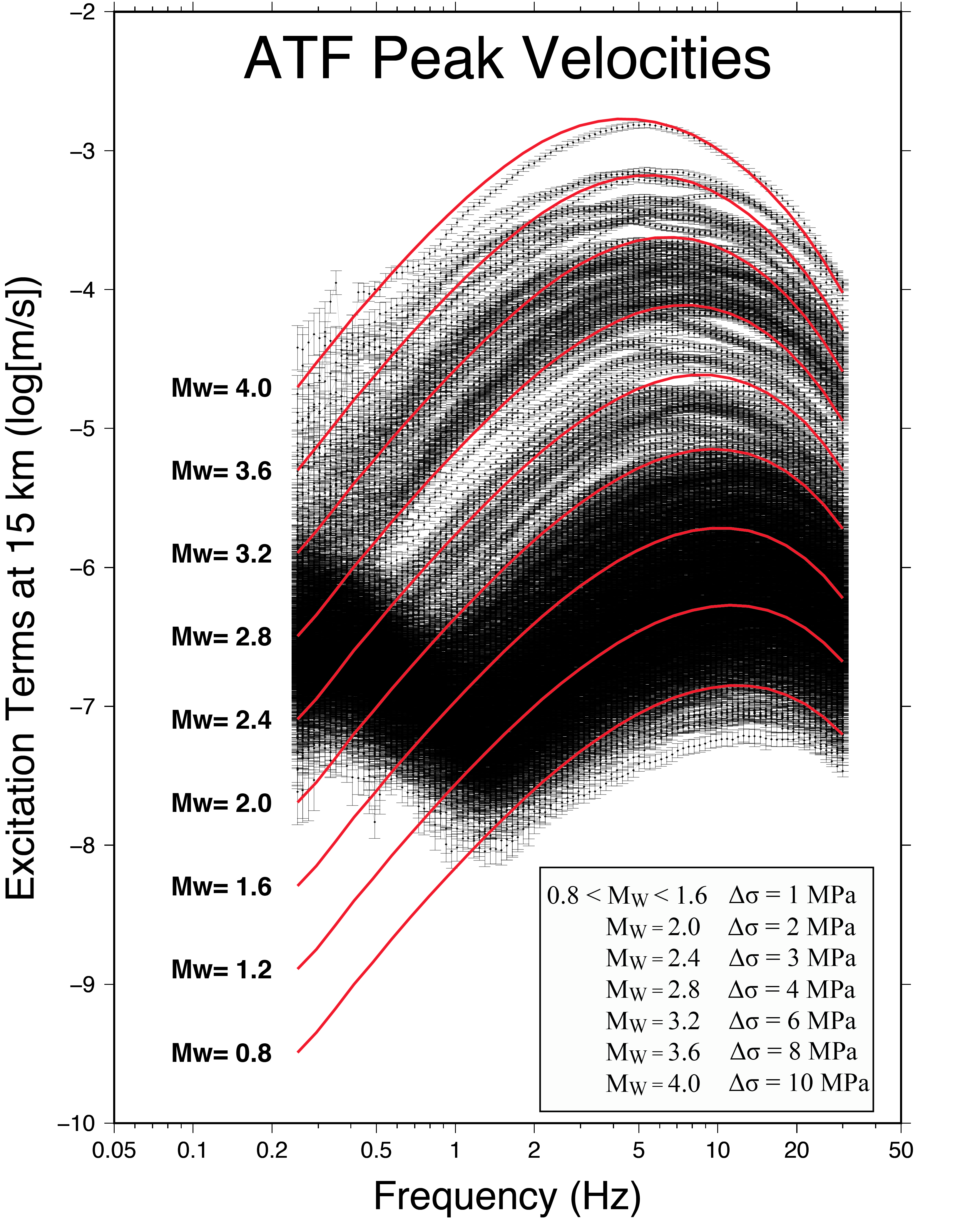
The empirical excitation terms SRCj(fi, r0) are modeled using the Brune (1970, 1971) spectral model; they describe the horizontal peak ground velocity as a function of frequency at the reference hypocentral distance of 15 km (Fig. S2). We fit the empirical excitation curves using random vibration theory (RVT; Cartwright and Longuet-Higgins, 1956), with the spectral model defined in equation (S3) and a duration function at the reference distance r0 that is the result of a regression (T = T(r = r0, fi); fref = 1.0 Hz in equation S2).
(S4)
The constant C in equation (S4) provides the right physical dimensions to the low-frequency spectral amplitudes, whereas the attenuation parameter k0 determines the high-frequency part of the synthetic spectra. Because the corner frequencies of small earthquakes may be outside the available bandwidth, k0 completely controls the behavior of the small earthquakes at high frequency.
To predict the seismic spectra, we used a single corner frequency Brune spectral model , with a stress drop varying as a function of magnitude between 1 MPa (at 0.8 < Mw < 1.6) and 10 MPa (at Mw = 4.0). The generic rock amplification function v(f) by Boore and Joyner (1997) is used in equation (S4), coupled with the parameter k0 = 0.035 s. The parameter Δσ is an effective stress parameter that does not necessarily represent the stress drop relaxed coseismically across the fault plane but that is needed to define, with a single corner frequency Brune spectrum, the spectral shapes of the empirical excitation terms.
The low-frequency content of the seismograms of our small earthquakes (fi < 1.0 Hz, Fig. S2) is contaminated by the microseismic noise at the average network site. Because of a constrain forced on our regressions (null average for the horizontal site terms), the low-frequency spectral bump that affects all the small source terms of Figure S2 is representative of the average noise level observed on all the horizontal components of the ground motion.
Table S1. All information about the earthquakes parameters of our data set (including event IDs, hypocentral coordinates, origin times, local magnitudes, moment magnitudes, seismic moments, and their standard deviations).
Figure S1. The empirical regional attenuation functional D(r, rref, f) obtained for the ATF region by regressing peak of the band-pass-filtered ground velocities at the sampling frequencies that are shown by colored lines. Black lines in the background represent the theoretical predictions. The attenuation function is normalized to zero at the reference hypocentral distance of 15 km. All lines are normalized by a 1/r decay (the horizontal dashed line represent the 1/r decay).
Figure S2. Source terms of 1191 events from the ATF data set (black lines). Red thick lines indicate the theoretical prediction at the indicated levels of moment magnitude from Brune source spectra coupled to the geometric-anelastic attenuation model.
Boore, D. M., and W. B. Joyner (1997). Site amplifications for generic rock sites, Bull. Seismol. Soc. Am. 87, 327–341.
Brune, J. N. (1970). Tectonic stress and the spectra of seismic shear waves from earthquakes, J. Geophys. Res. 75, 4997–5009.
Brune, J. N. (1971). Correction, J. Geophys. Res. 76, 5002.
Cartwright, D. E., and M. S. Longuet-Higgins (1956). The statistical distribution of the maxima of a random function, Proc. Roy. Soc. Lond. 237, 212–232.
Malagnini, L., and D. Dreger (2016). Generalized free-surface effect and random vibration theory: A new tool for computing moment magnitudes of small earthquakes using borehole data, Geophys. J. Int. 206, no. 1, 103–113, doi: 10.1093/gji/ggw113.
[ Back ]