This electronic supplement contains figures showing calculated Pn-wave spectral amplitudes versus distance.
Calculated Pn-wave spectral amplitudes versus distance are shown for suites of models with random velocity heterogeneity realizations from Table 1 of the main article. Results for each of eight models are shown in Figures S1–S8. Comparisons of results with individual heterogeneity parameters varying are shown in Figures S9–S11.
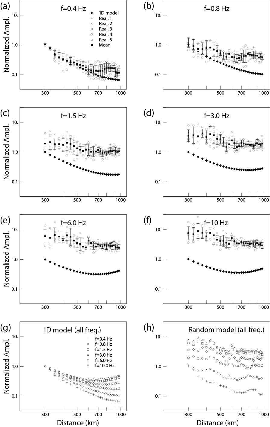
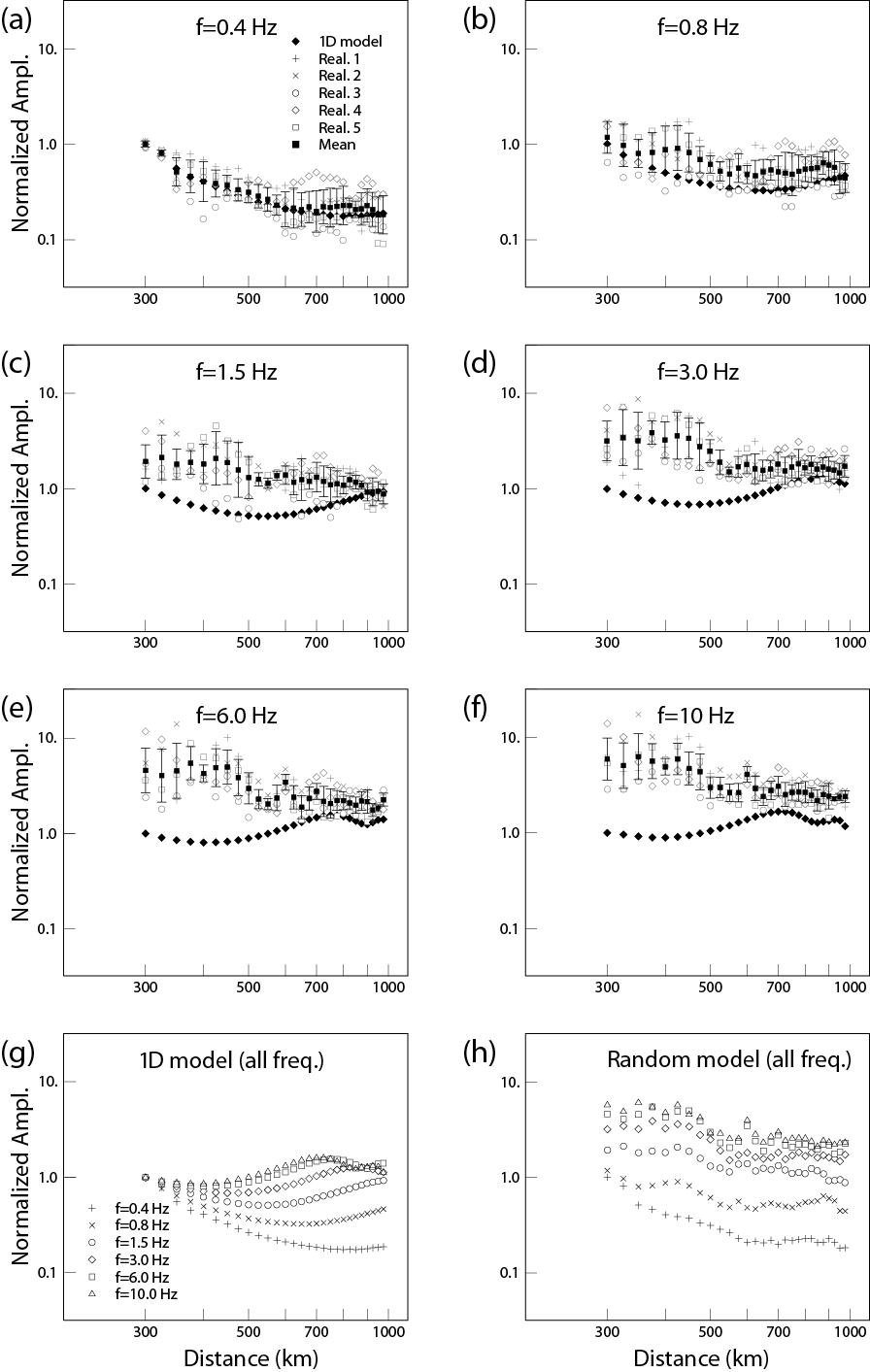
Figure S1. Pn-wave spectral amplitude versus distance calculated from random velocity model 2 in Table 1 of the main article. (a)–(f) are spectral amplitudes at 0.4, 0.8, 1.5, 3.0, 6.0, and 10 Hz. (g) Amplitudes in the 1D background model. Different symbols are for different frequencies. (h) Mean amplitudes for the random velocity model.
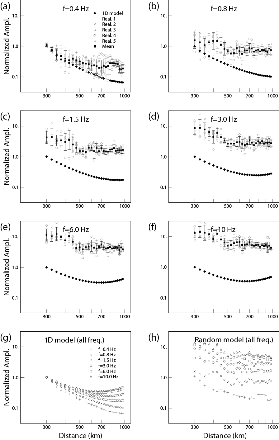
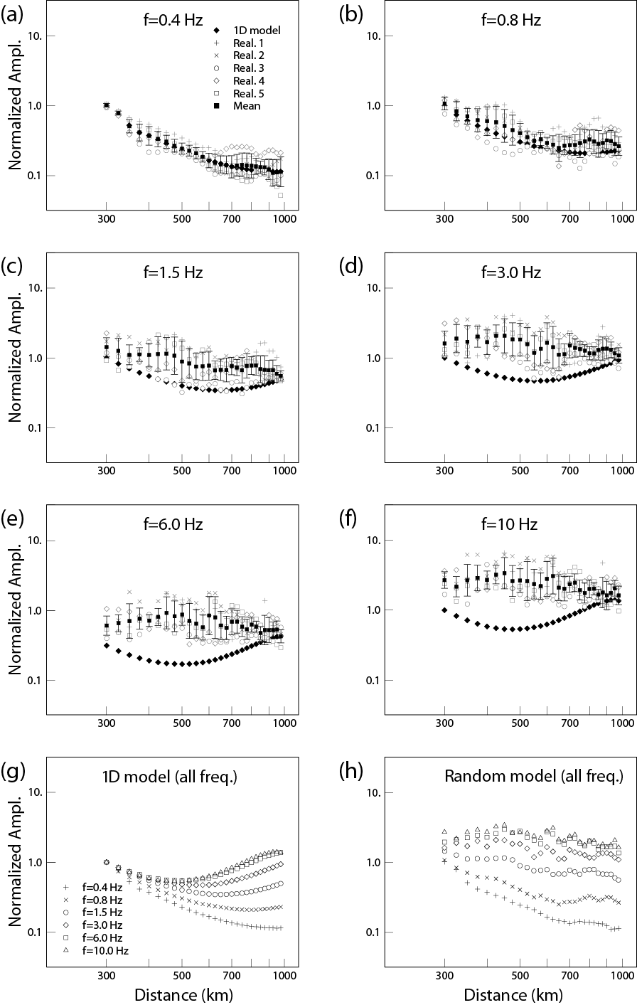
Figure S2. Pn-wave spectral amplitude versus distance calculated from random velocity model 3 in Table 1 of the main article. (a)–(f) are spectral amplitudes at 0.4, 0.8, 1.5, 3.0, 6.0, and 10 Hz. (g) Amplitudes in the 1D background model. Different symbols are for different frequencies. (h) Mean amplitudes for the random velocity model.
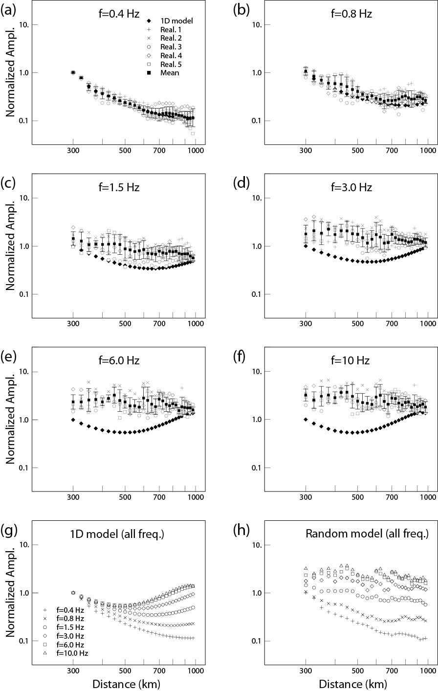
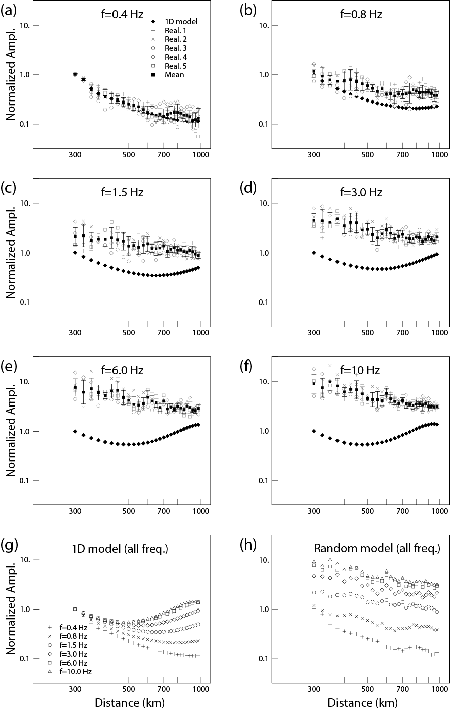
Figure S3. Pn-wave spectral amplitude versus distance calculated from random velocity model 4 in Table 1 of the main article. (a)–(f) are spectral amplitudes at 0.4, 0.8, 1.5, 3.0, 6.0, and 10 Hz. (g) Amplitudes in the 1D background model. Different symbols are for different frequencies. (h) Mean amplitudes for the random velocity model.
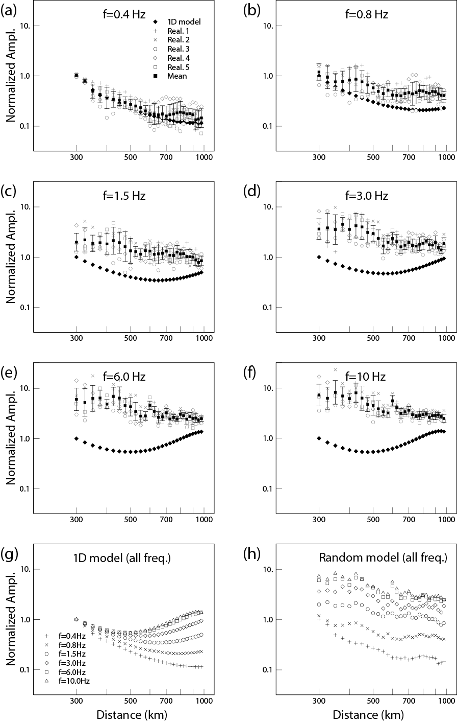
Figure S4. Pn-wave spectral amplitude versus distance calculated from random velocity model 5 in Table 1 of the main article. (a)–(f) are spectral amplitudes at 0.4, 0.8, 1.5, 3.0, 6.0, and 10 Hz. (g) Amplitudes in the 1D background model. Different symbols are for different frequencies. (h) Mean amplitudes for the random velocity model.
Figure S5. Pn-wave spectral amplitude versus distance calculated from random velocity model 6 in Table 1 of the main article. (a)–(f) are spectral amplitudes at 0.4, 0.8, 1.5, 3.0, 6.0, and 10 Hz. (g) Amplitudes in the 1D background model. Different symbols are for different frequencies. (h) Mean amplitudes for the random velocity model.
Figure S6. Pn-wave spectral amplitude versus distance calculated from random velocity model 7 in Table 1 of the main article. (a)–(f) are spectral amplitudes at 0.4, 0.8, 1.5, 3.0, 6.0, and 10 Hz. (g) Amplitudes in the 1D background model. Different symbols are for different frequencies. (h) Mean amplitudes for the random velocity model.
Figure S7. Pn-wave spectral amplitude versus distance calculated from random velocity model 8 in Table 1 of the main article. (a)–(f) are spectral amplitudes at 0.4, 0.8, 1.5, 3.0, 6.0, and 10 Hz. (g) Amplitudes in the 1D background model. Different symbols are for different frequencies. (h) Mean amplitudes for the random velocity model.
Figure S8. Pn-wave spectral amplitude versus distance calculated from random velocity model 9 in Table 1 of the main article. (a)–(f) are spectral amplitudes at 0.4, 0.8, 1.5, 3.0, 6.0, and 10 Hz. (g) Amplitudes in the 1D background model. Different symbols are for different frequencies. (h) Mean amplitudes for the random velocity model.
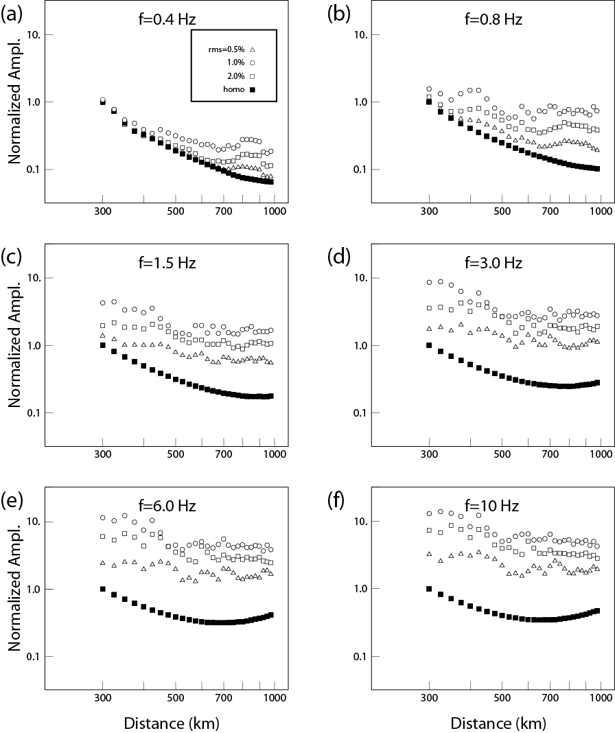
Figure S9. Comparison between Pn-wave spectral amplitudes calculated from random velocity models 1, 2, and 3 in Table 1 of the main article. These models have the same velocity gradient and random parameters but different root mean square (rms) velocity perturbations. Open triangles, circles, and squares are for models with 0.5%, 1.0%, and 2.0% velocity perturbations, respectively. The solid squares are for the background model. (a)–(f) are for spectral amplitudes at individual frequencies.
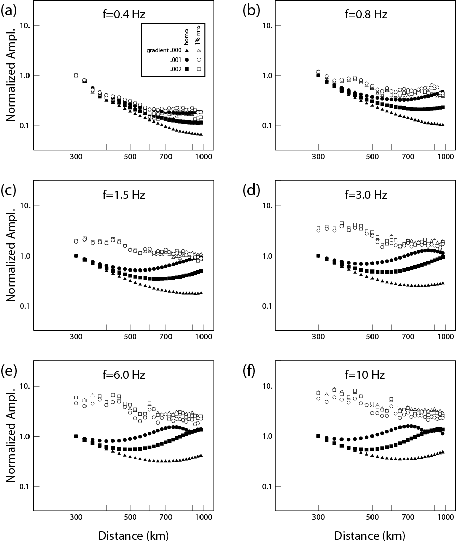
Figure S10. Comparison between Pn-wave spectral amplitudes calculated from random velocity models 2, 5, and 6 in Table 1 of the main article. These models have the same horizontal and vertical correlation lengths 20 and 6 km, and rms velocity perturbation of 1%, but the velocity gradients are different. Triangles, circles, and squares are for models with velocity gradients 0.000, 0.001, and 0.002. The open symbols are for random velocity models, and solid symbols are for related background velocity models. (a)–(f) are for spectral amplitudes at individual frequencies.
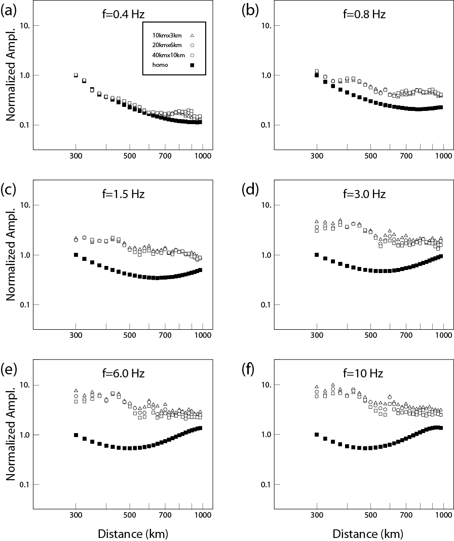
Figure S11. Comparison between Pn-wave spectral amplitudes calculated from random velocity models 5, 8, and 9 in Table 1 of the main article. These models have the same upper-mantle velocity gradients of 0.001, the same rms velocity perturbation of 1%, but their horizontal and vertical correlation lengths are different. (a)–(f) are for spectral amplitudes at individual frequencies. The open triangles, circles, and squares are for models with correlation lengths 10 km × 3 km, 20 km × 6 km, and 40 km × 10 km. The solid squares are for the related background model.
[ Back ]