This electronic supplement contains histograms of synthetic peak ground accelerations (PGAs) and peak ground velocities (PGVs), providing a detailed representation of the synthetic ground-motion distributions for each magnitude and distance pairs considered in our analyses.
For Mw 7.0 and 6.0, based on visual inspection and statistical tests (i.e., Kolmogorov–Smirnov test and χ-square test with 5% confidence interval), the synthetic PGA follows, on average, a lognormal distribution, independently of the modeling setup (M1, M2, and M3). However, directivity effects can generate distributions characterized by either positive or negative skew (e.g., the PGA distributions at s001 relative to the Mw 7.0 case). Compared to the PGAs, the PGV values are better described by multimodal distributions. For the Mw 5.0 case we observe that, independently from the scenario model, the ground-motion parameter distributions can be only approximated by lognormal shapes both at high and at low frequencies; a larger number of child faults (CFs) should be considered to better sample the parent fault (PF) to generate a lognormal distribution.
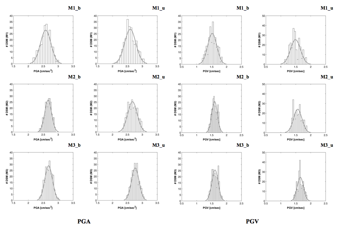
Figure S1. Histograms of the synthetic PGA and PGV (alternate columns) for Mw 7.0 and RJB = 0 km, fitted by a normal distribution (gray line). Statistical distributions are for different scenario configurations: uppermost panels: finite-fault simulations with apparent corner frequency (M1); central panels: point-source simulations (M2); and lowermost panels: merging between finite-fault and point-source simulations imposing a corner frequency threshold of 0.07 Hz (M3). Simulations were performed both at the bilateral site (_b = CSZ) and at the quasi-unilateral site (_u = s001).
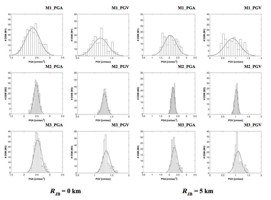
Figure S2. Histograms of the synthetic PGA and PGV (alternate columns) for Mw 6.0 with respect to the city of Cosenza (CSZ) site fitted by a normal distribution (gray line). Leftmost two columns: RJB = 0 km; rightmost two columns: average RJB = 5 km. Statistical distributions are for different scenario configurations: uppermost panels: finite-fault simulations with apparent corner frequency (M1); central panels: point-source simulations (M2); and lowermost panels: merging between finite-fault and point-source simulations imposing a corner frequency threshold of 0.23 Hz (M3).
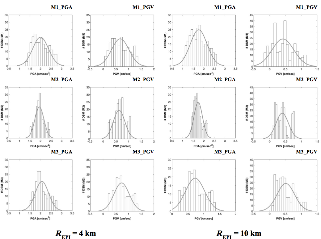
Figure S3. Histograms of the synthetic PGA and PGV (alternate columns) for Mw 5.0 with respect to the CSZ site fitted by a normal distribution (gray line). Leftmost two columns: average Repi = 4 km; rightmost two columns: average Repi = 10 km. Statistical distributions are for different scenario configurations: uppermost panels: finite-fault simulations with apparent corner frequency (M1); central panels: point-source simulations (M2); and lowermost panels: merging between finite-fault and point-source simulations imposing a corner frequency threshold of 0.7 Hz (M3).
[ Back ]