This electronic supplement contains a description of the smoothing process applied to the original 3D velocity model, 11 figures (Figs. S1–S11), and a movie (Movie S1). Most of the material focuses on the alternative fault geometry (Wei et al., 2015) considered in the main article. It also contains results for a couple of tests in which we tapered the inverted slip model and neglected three stations in the inversion. Waveform predictions at several stations not included in the inversion and vertical profiles of the 3D velocity models are shown as well. Finally, we include a movie showing wave propagation in the U.S. Geological Survey (USGS) 3D velocity model (USGSBayAreaVM-08.3.0.etree; see Data and Resources).
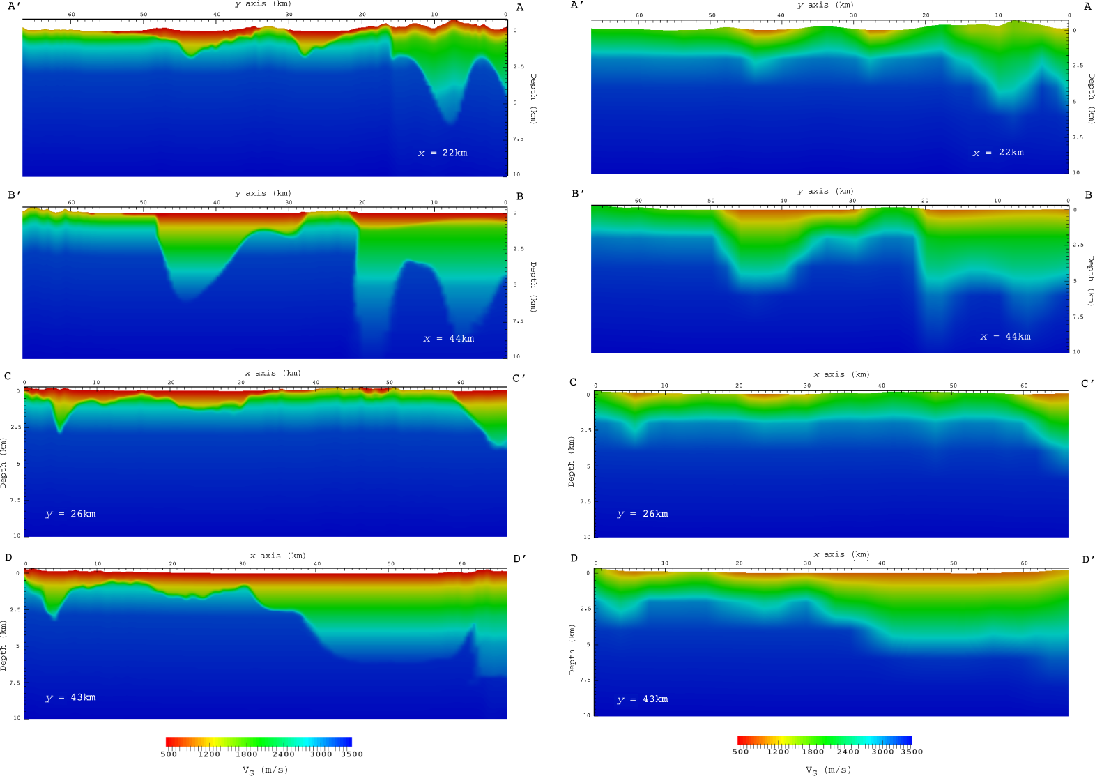
The smoothing of the original 3D velocity model is realized on a regular grid with points 2 km apart. For each point, a single value for velocity, density, and attenuation is computed by averaging all values in the original USGS velocity model found within 1 km distance, in all directions, from the point. Velocity values are not clipped before averaging. Also, points located above topography or in the water are excluded from the calculations. This coarse velocity model is then interpolated onto the finer finite-difference grid. Vertical profiles of either original or smoothed 3D velocity models are shown in Figure S11.
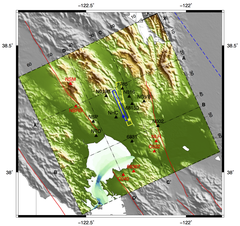
Figure S1. Map of the area under study showing stations (triangles), fault projections, and epicenters for each fault model (Gallovič, blue; Wei, yellow), together with a schematic representation of main faults in the Bay area (red lines). The colored area defines the numerical domain for finite-difference calculations, for which dimensions are reported in kilometers. Black dashed lines and letters indicate locations of cross sections shown in Figure S11. Note that the stations in red were not used in the source inversion but only for the forward waveform prediction in Figure S7.
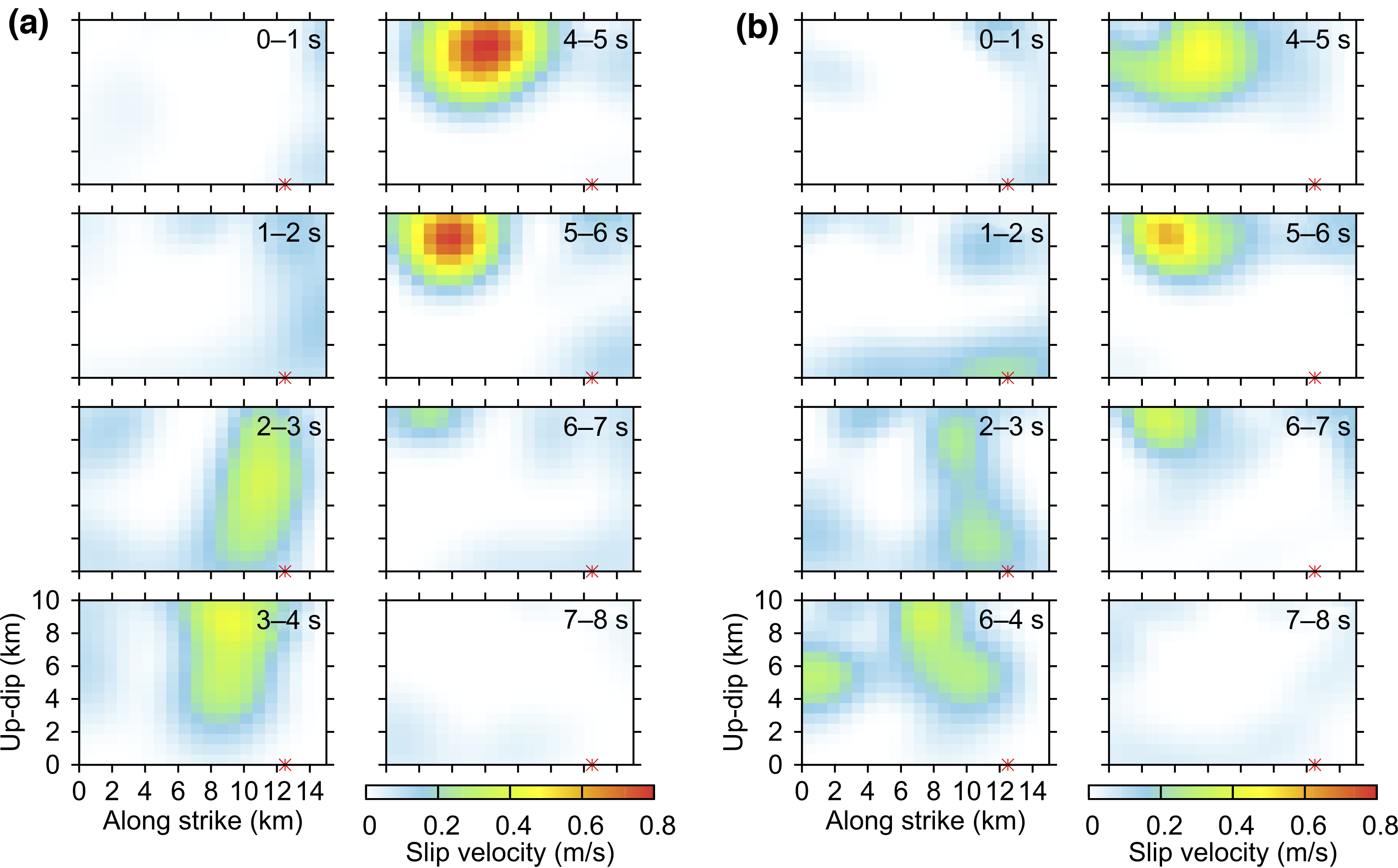
Figure S2. Snapshots of the rupture process as obtained by slip inversion considering the Gallovič (2016) fault geometry and using (a) 1D and (b) 3D Green’s functions (GFs). Note that the latter is characterized by unphysical features with respect to the former, such as the relatively large slip velocity close to the left edge of the fault at 3–4 s.
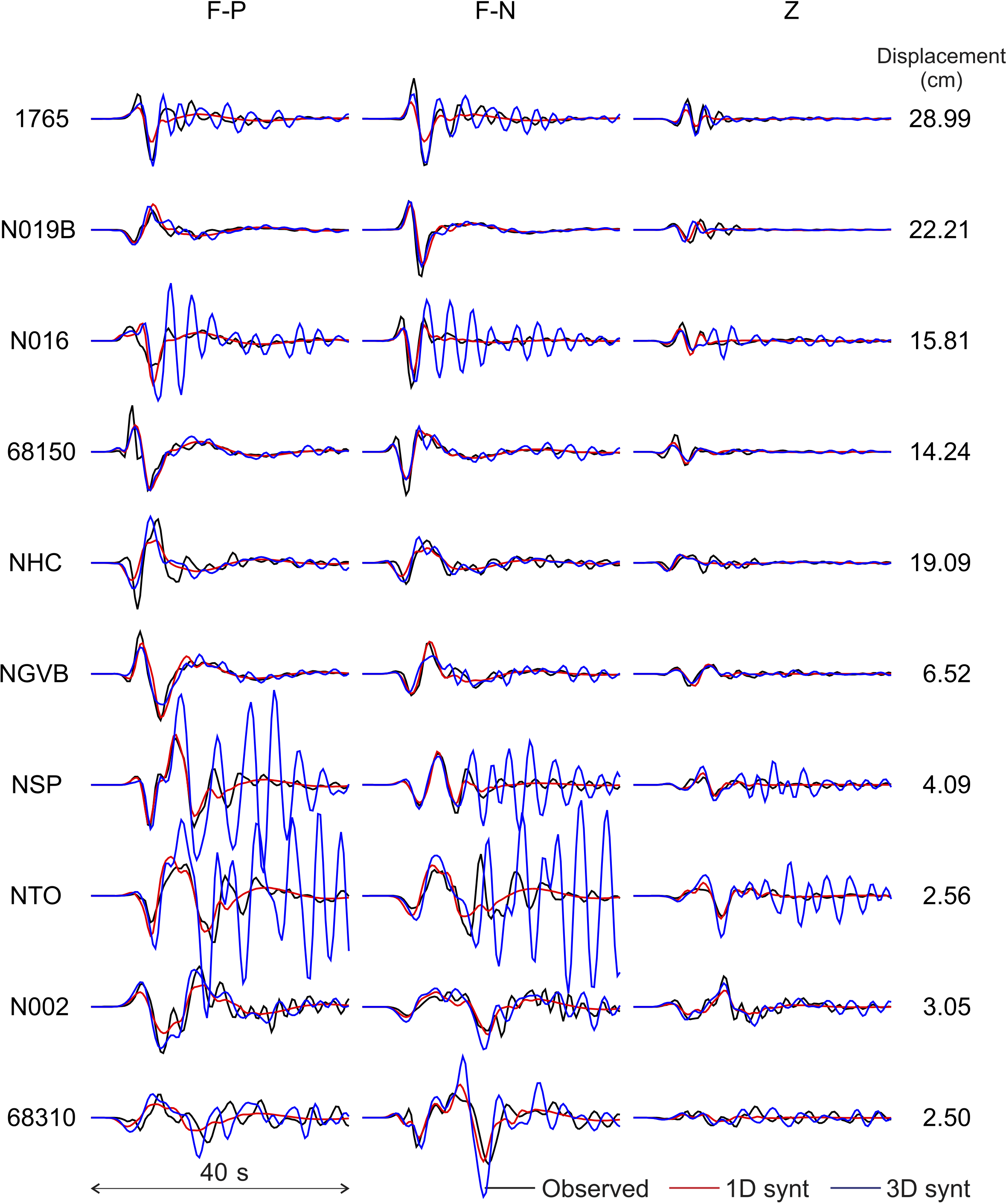
Figure S3. Comparison between observed (black) and synthetic seismograms for the Gallovič (2016) fault model forward calculated using the 1D GF source model and 1D (red) or 3D (blue) GFs. Note the large oscillations at several stations not observed in the recorded data.
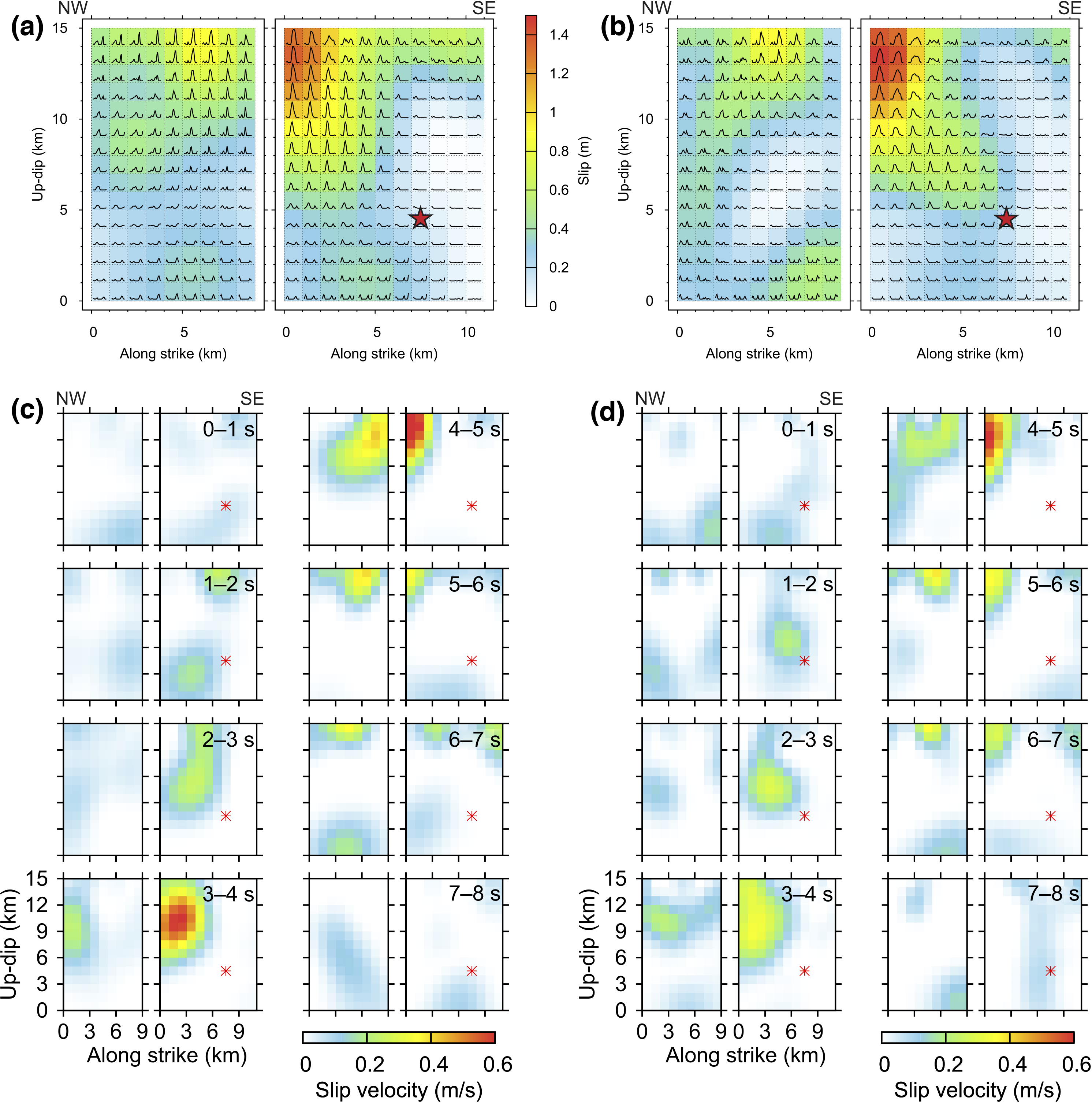
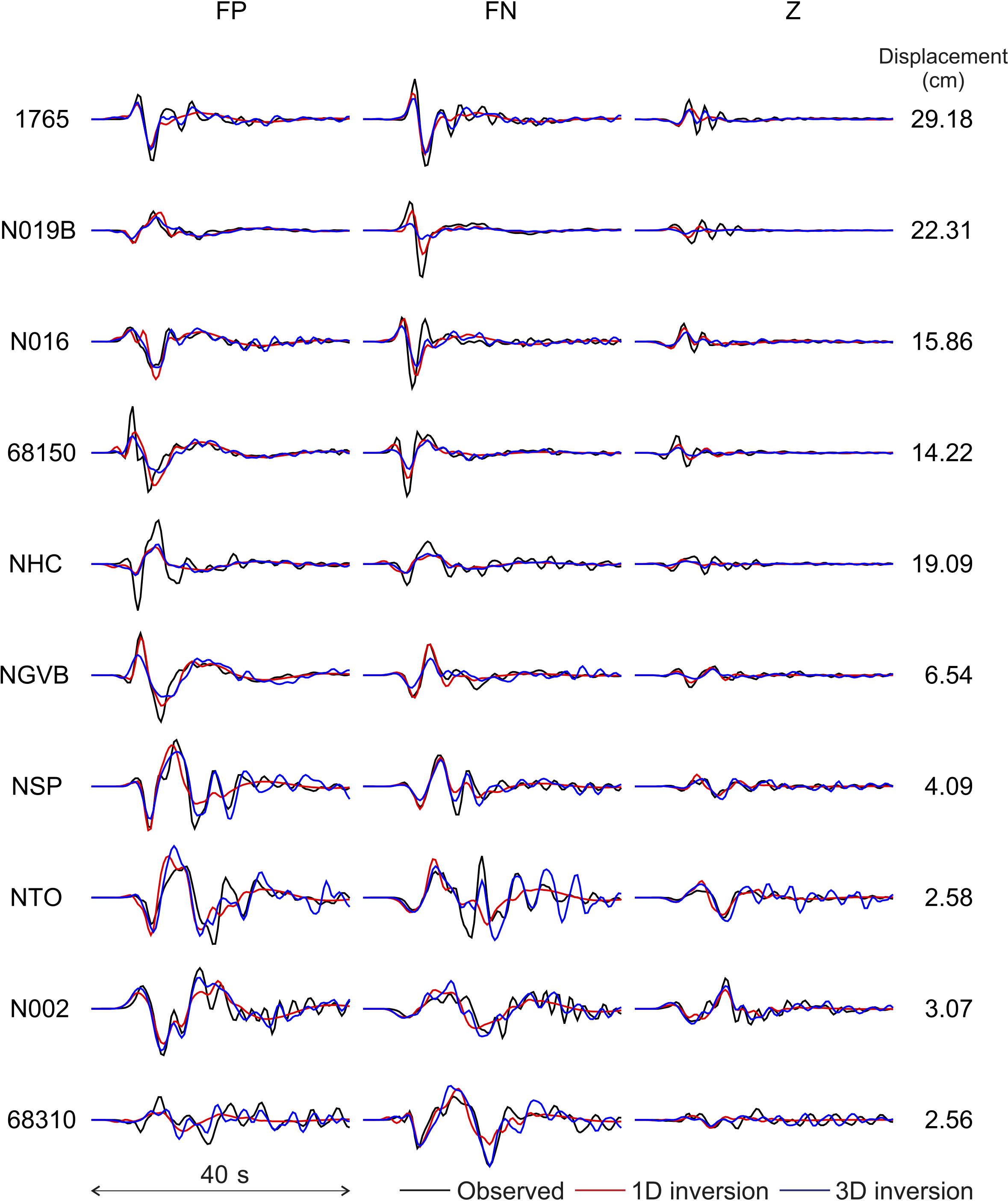
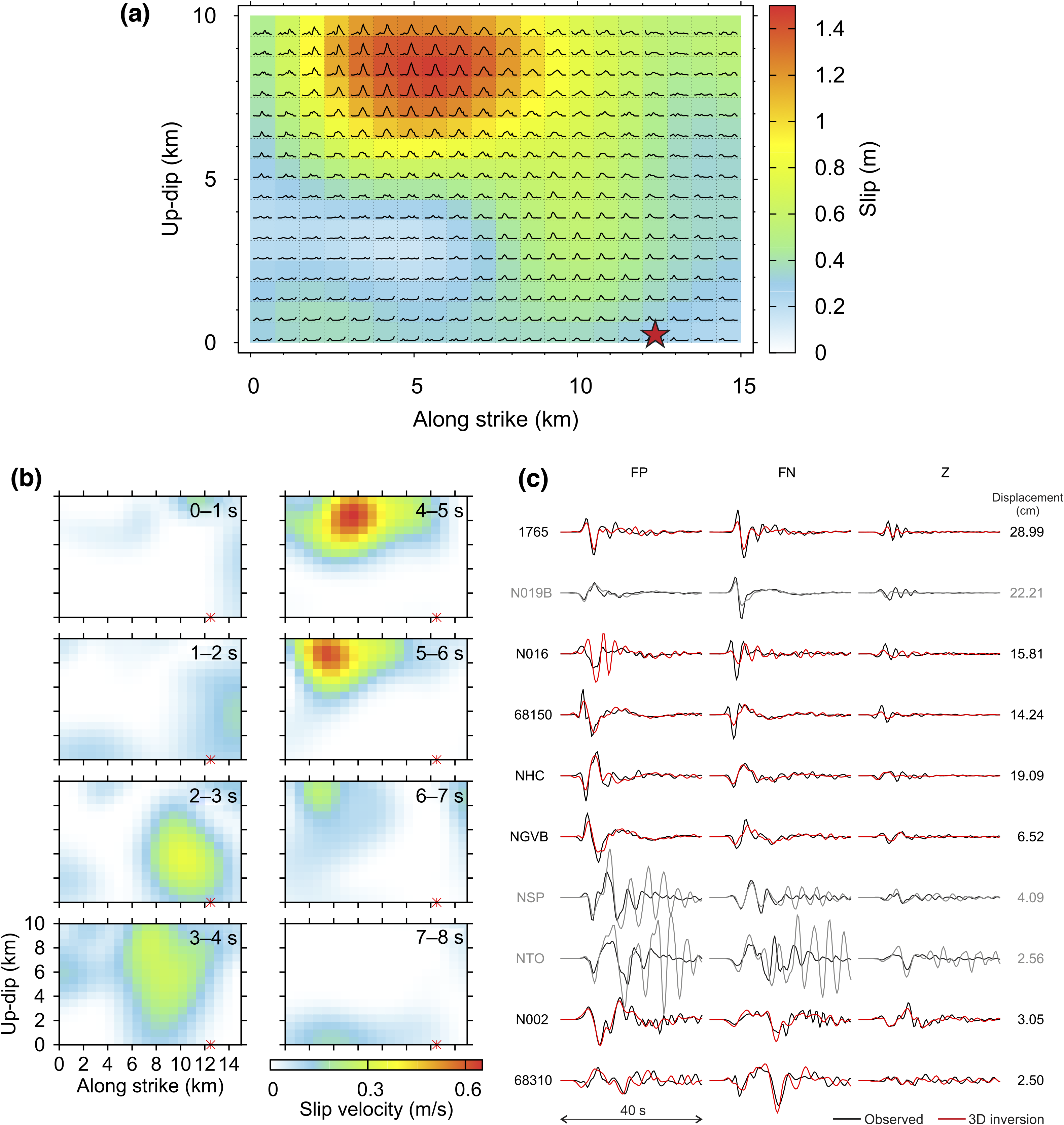
Figure S4. Inversion results for the Wei et al. (2015) two-segment fault model. (Top) Slip distributions and slip-rate functions inferred considering the (a) 1D and (b) 3D velocity models. The duration of the slip rates is limited to the first 8 s after the rupture initiates at the hypocenter (red star). (c,d) Snapshots showing the evolution of the rupture front for each of the two cases. Waveform comparison for these two models is shown in Figure S5.
Figure S5. Comparison between observed (black) and synthetic displacement waveforms (0.05–0.5 Hz) for the source models shown in Figure S4 (Wei et al., 2015, fault geometry) inverted using the 1D (red) and 3D (blue) GFs, respectively. Generally speaking, in the 3D inversion the waveform fit for the later arrivals at distant stations improves with respect to the 1D inversion, whereas it worsens for the first main pulses at the nearest stations.
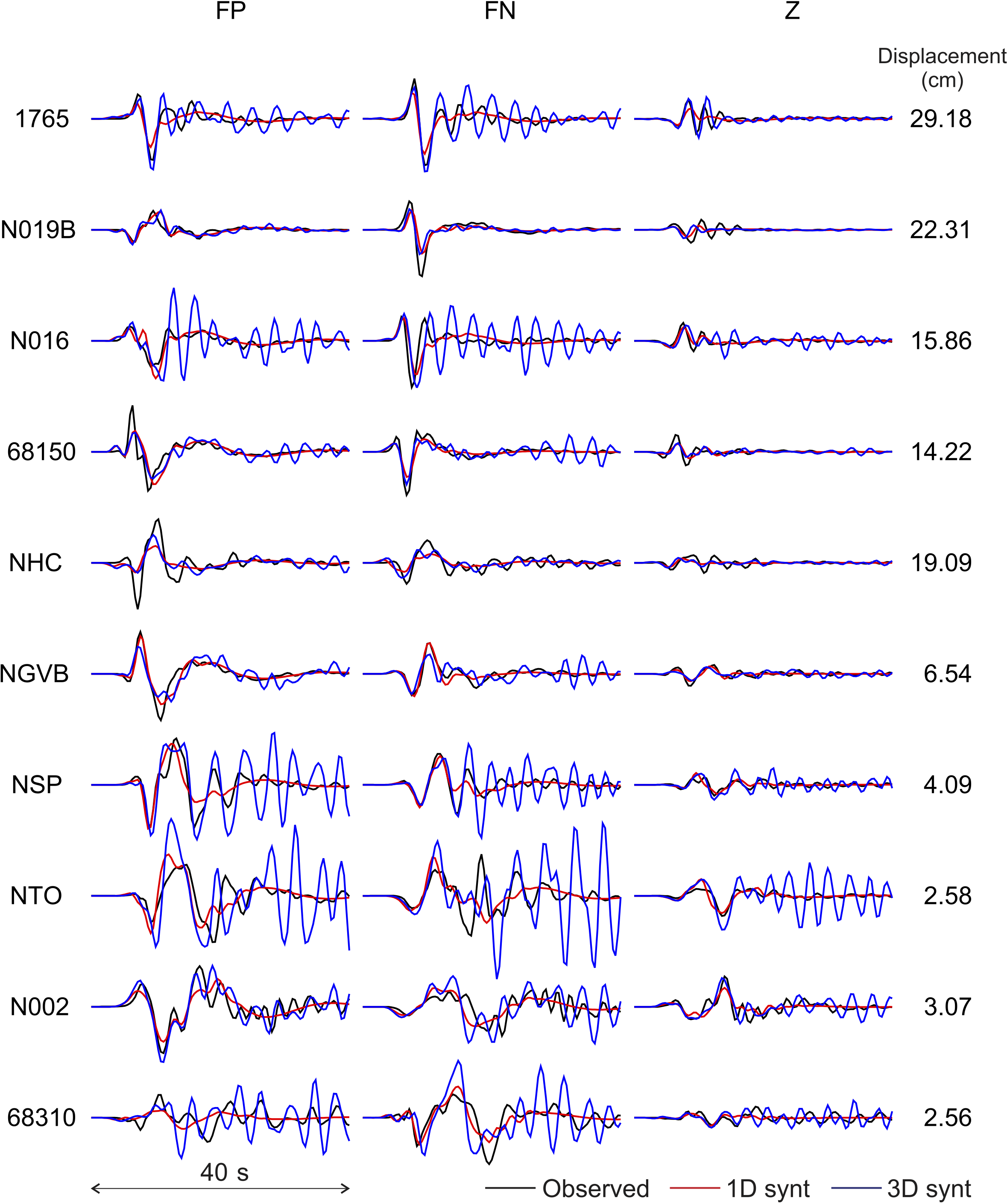
Figure S6. Comparison between observed (black) and synthetic seismograms for the Wei et al. (2015) fault model forward calculated using the 1D GF source model and 1D (red) or 3D (blue) GFs. Note the large oscillations at several stations not observed in the recorded data, which are present also in the analogous test using the Gallovič (2016) fault geometry (see Fig. 1b in the main article and Fig. S3).
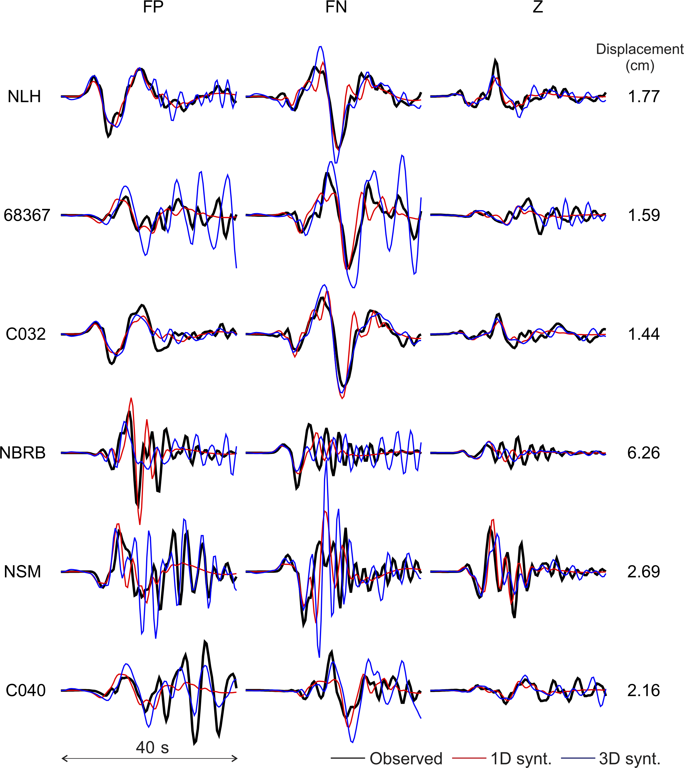
Figure S7. Comparison between observed (black) and synthetic seismograms for the Gallovič (2016) fault model computed using the 1D GF source model and 1D (red) or 3D (blue) GFs at receivers not included in the inversion procedure (see Fig. S1). Large-amplitude oscillations not recorded in the data may be observed mainly at receiver 68367.
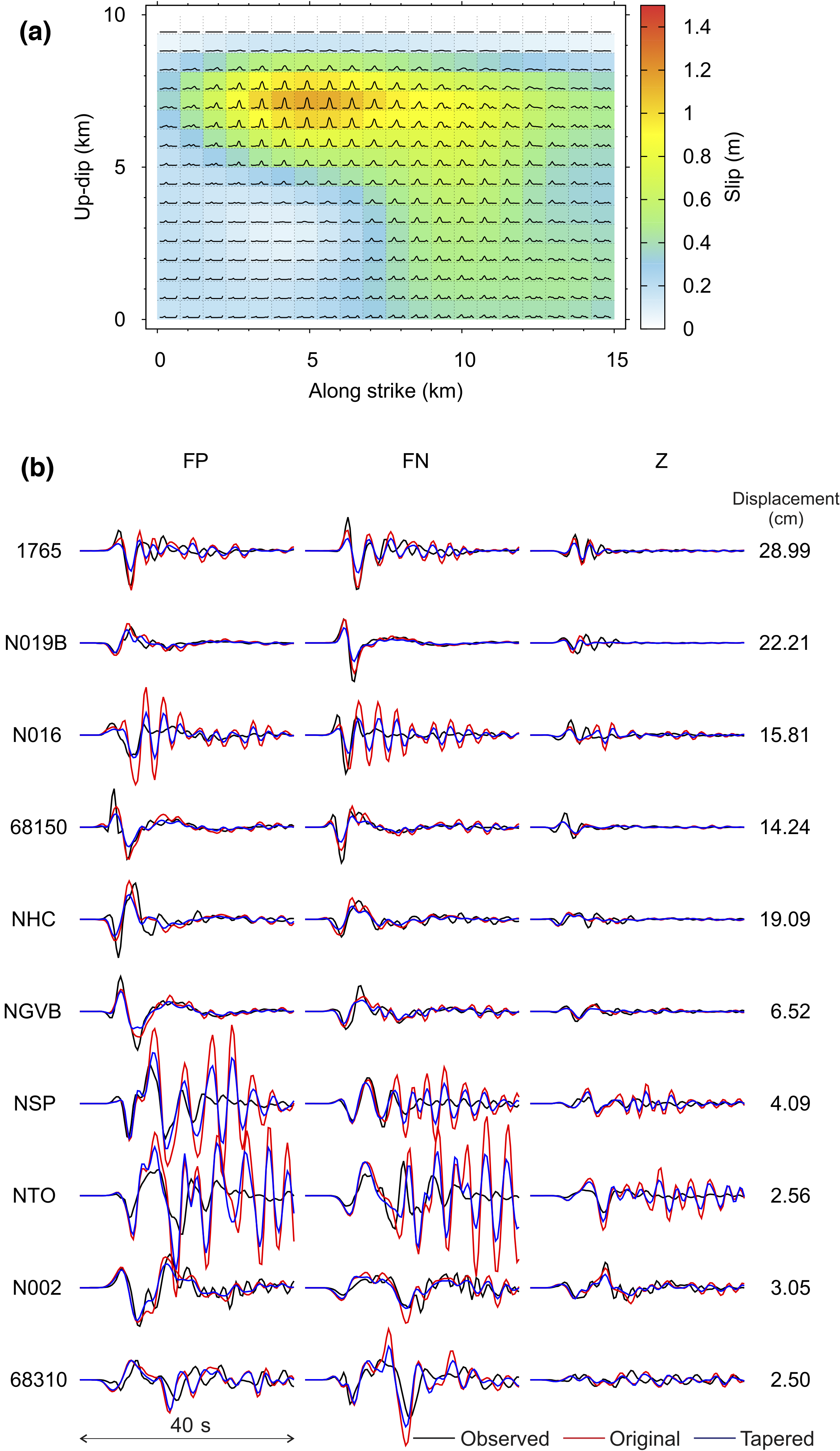
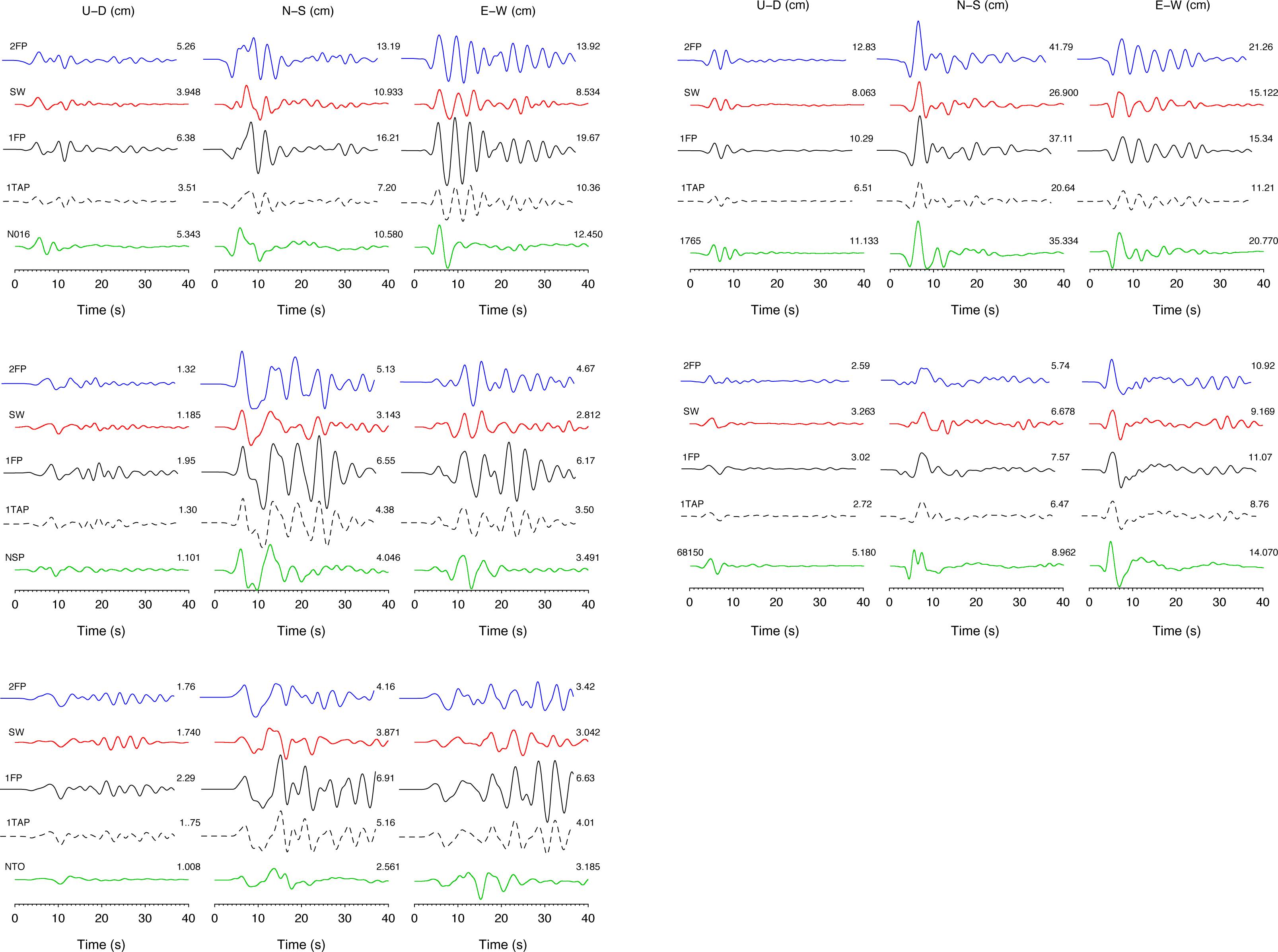
Figure S8. (a) Artificially tapered source model used to test the effect of the shallowest subfaults on the waveforms. (b) Observed (black) and synthetic seismograms computed using the original (red) and tapered (blue) source model. Both set of synthetics are referred to the 3D velocity model. Note that the tapering does not fully suppress the strong surface waves.
Figure S9. Comparison between recorded seismograms (green), original synthetics of Wei et al. (2015) (red, labeled as SW), and our synthetics computed using the 3D velocity model and our 1D GF source models: Wei et al. (2015) fault geometry (blue, labeled as 2FP), Gallovič (2016) fault geometry (black, labeled as 1FP), and Gallovič (2016) fault geometry with slip tapering (dashed black, labeled as 1TAP). Only receivers N016, NSP, NTO, 1765, and 68150 are shown. All synthetics present late oscillations larger than observed.
Figure S10. (a) Slip distribution and slip-rate functions as inferred from the inversion based on the 3D GFs after excluding receivers NSP, NTO, and N016, considering the Gallovič (2016) fault geometry. The duration of the slip rates is limited to the first 8 s after the rupture initiates at the hypocenter (red star). (b) Snapshots showing the evolution of rupture front. (c) Waveform fit. Note that synthetics at receivers NSP, NTO, and N016 (in gray) are computed separately after the inversion using the 3D GFs.
Figure S11. Vertical cross sections of the 3D USGS velocity model (a) before and (b) after smoothing across the simulation domain. Note the faster shallow sediments and the more diffuse interfaces after the smoothing. Location of the cross sections is shown in Figure S1.
Movie S1 [JPEG2000-encoded MPEG4 movie; ~6.3 MB]. Magnitude of ground-motion velocity (0.05–0.5 Hz) computed for the 1D GF source model embedded in the USGS 3D velocity model before (left) and after (right) smoothing. Both topography and intrinsic attenuation are included in the calculations.
The U.S. Geological Survey (USGS) 3D seismic velocity model v.8.3 is available at http://earthquake.usgs.gov/data/3dgeologic/download.php (last accessed April 2016).
Gallovič, F. (2016). Modeling velocity recordings of the Mw 6.0 South Napa, California, earthquake: Unilateral event with weak high-frequency directivity, Seismol. Res. Lett. 87, 2–14.
Wei, S., S. Barbot, R. Graves, J. J. Lienkaemper, T. Wang, K. Hudnut, Y. Fu, and D. Helmberger (2015). The 2014 Mw 6.1 South Napa earthquake: A unilateral rupture with shallow asperity and rapid afterslip, Seismol. Res. Lett. 86, 344–354.
[ Back ]