This electronic supplement contains figures illustrating a reconstructed slice showing the Red Fork sand formation in the Prague area (Fig. S1), additional recorded waveforms from the aftershocks (Figs. S2–S4), a Wadati diagram (Fig S5), the complete velocity model used for the calculation (Fig. S6) and map of synthetic seismographs (Fig. S7), and time slices generated by the finite-difference wavefield model (Figs. S8 and S9); and tables summarizing locations of the seismometers (Table S1), statistical constrains used for modeling the paleochannels (Table S2), and details of the relocated hypocenters (Table S3).
Table S1. List of three-component seismograph stations used in the study.
Table S2. Normally distributed constraints of the modeled paleochannels. The dimensions of the channels are learnt from investigations by Joseph (1986).
Table S3. Relocations of 13 aftershocks from the 2011 Oklahoma earthquake sequence based on a gradient, half-space model.
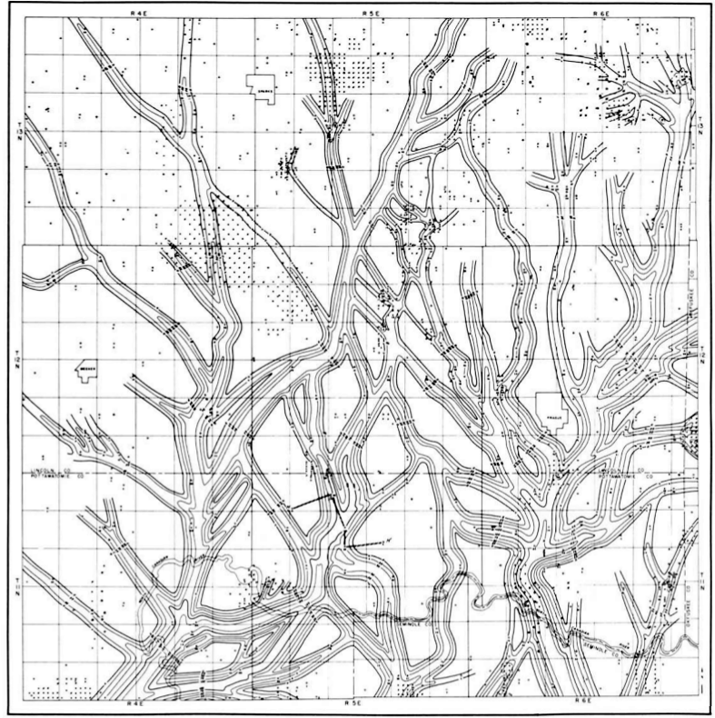
Figure S1. Map showing the reconstruction of paleochannels in the Red Fork Sand Formation within the Pennsylvanian marine limestone group, around the study area of Prague, Oklahoma. Thickly framed area plots indicate township and range blocks, measuring 6 × 6 miles. Each township and range block is further divided into 36 sections, measuring 1 × 1 miles. This work is interpreted from numerous well logs from the region. Adapted from Joseph (1986).
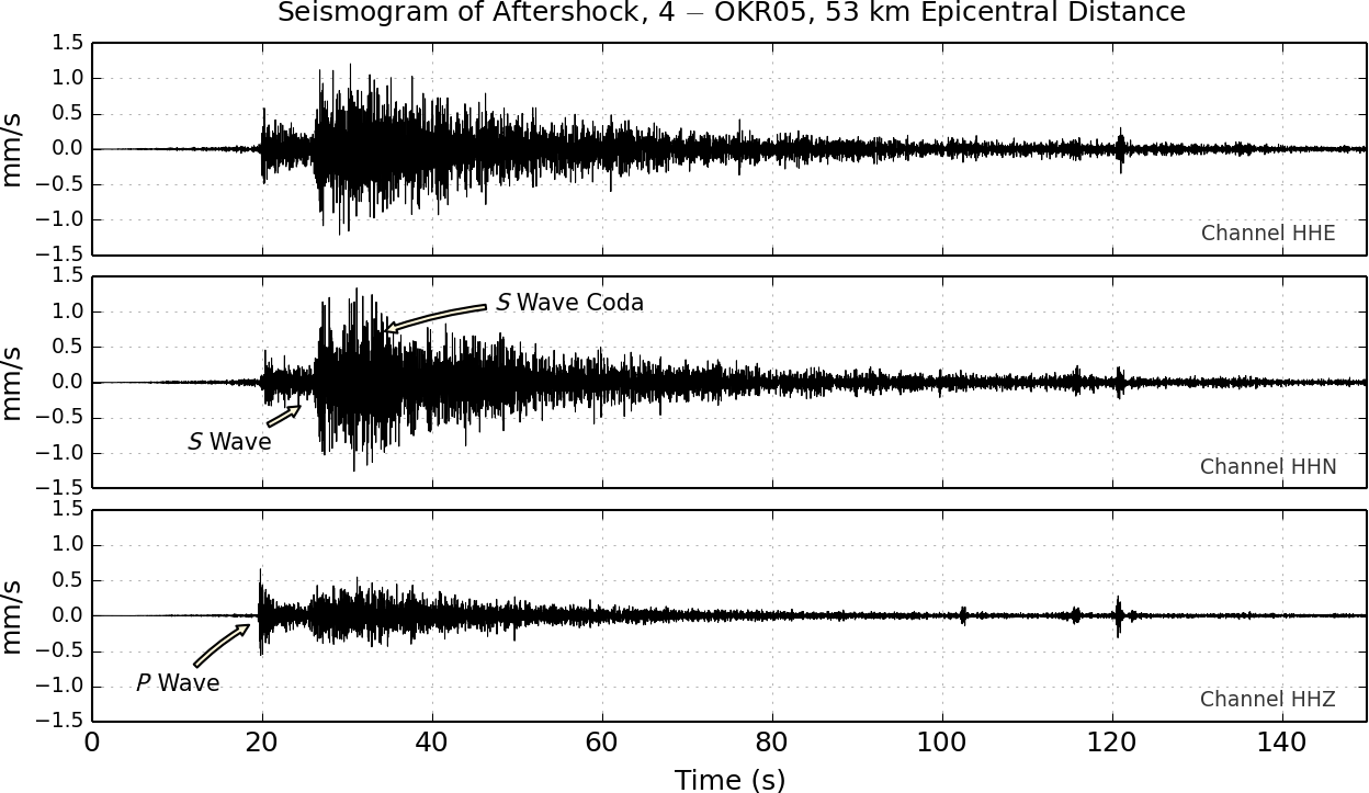
Figure S2. Three-component seismogram of aftershock 4, ML 3.2, focal depth 7.15 km at 53 km epicentral distance from station LA.OKR05. The arrival of the direct P and S waves can be observed on all components. Both phases are followed by a prominent wave coda, in which the S wave coda is particularly visible on the horizontal components of the seismogram.
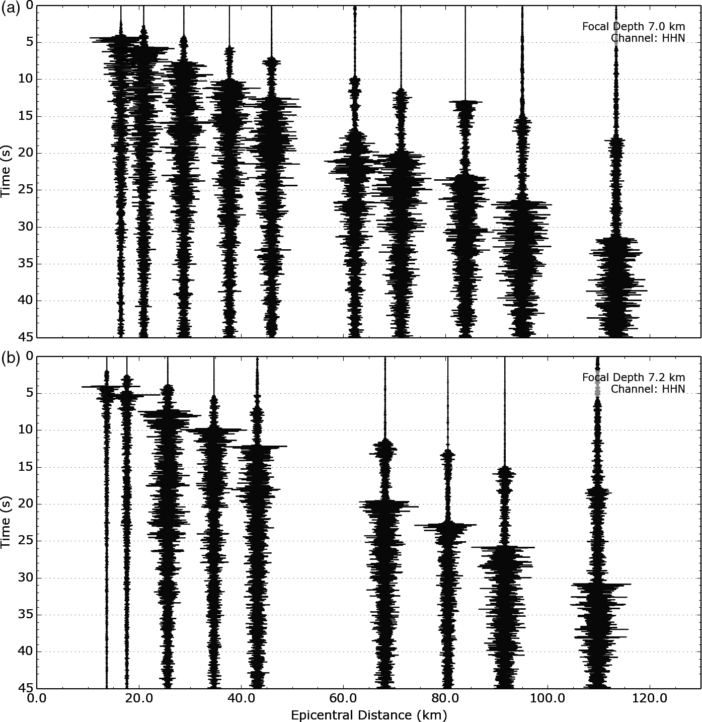
Figure S3. Record sections recorded by the large aperture (LA) network, horizontal component. (a) Aftershock 3: ML 3.2, depth 7.0 km; and (b) aftershock 5: ML 3.2, depth 7.2 km. The data are high-pass filtered f > 0.5 Hz.
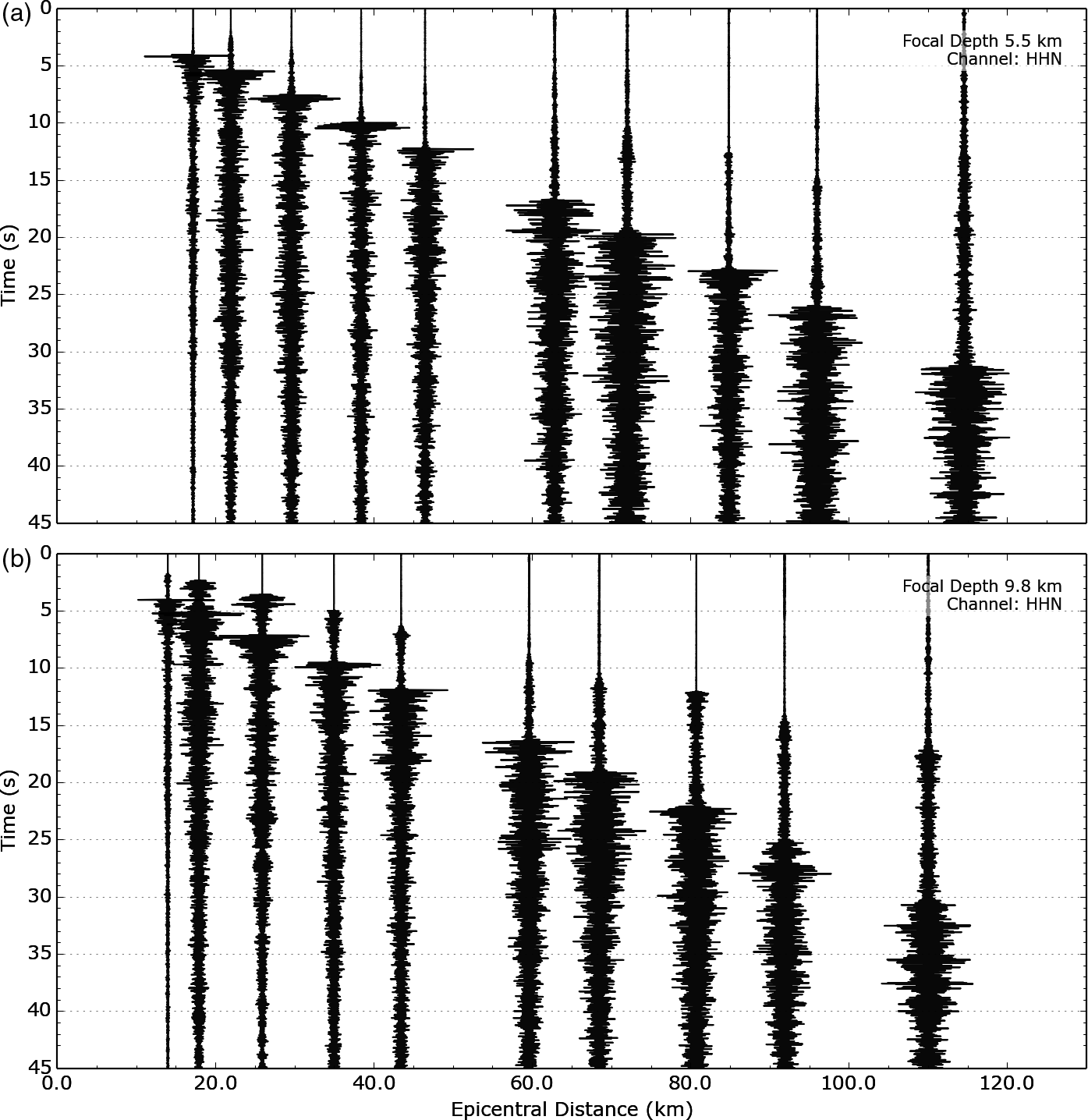
Figure S4. Record sections recorded by the LA network, horizontal component. (a) Aftershock 6: ML 3.2, depth 5.5 km; and (b) aftershock 7: ML 3.3, depth 9.8 km. The data are high-pass filtered f > 0.5 Hz.
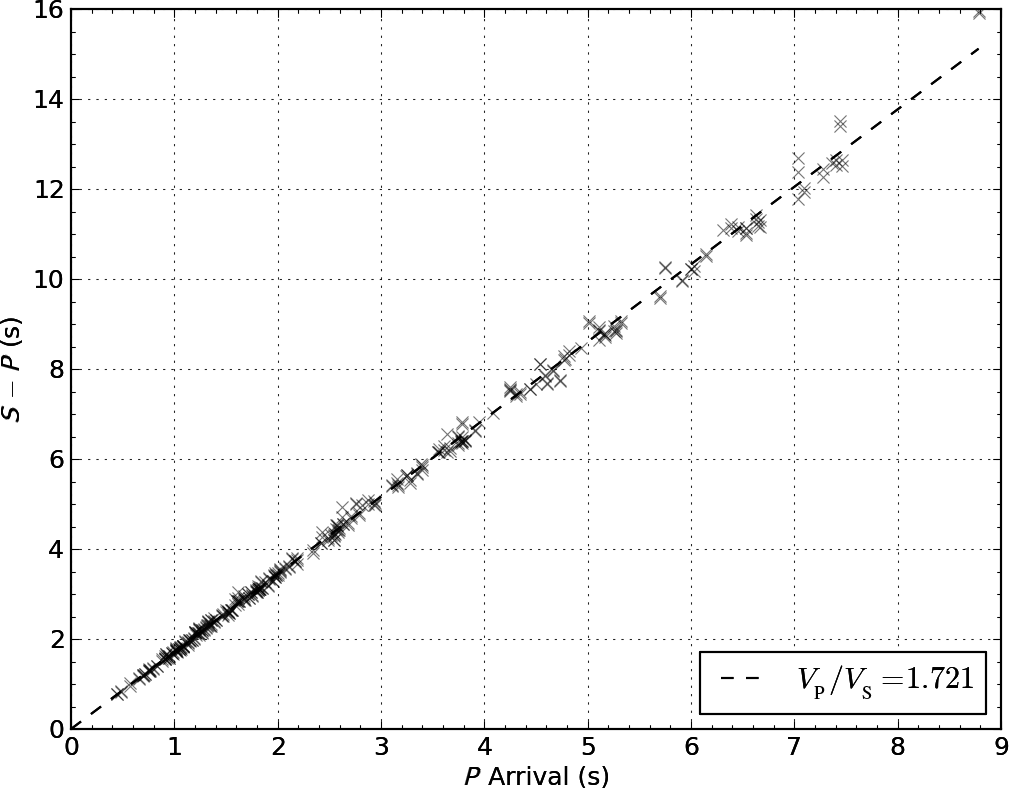
Figure S5. Wadati diagram of P and S waves relative arrival times of 16 aftershocks picked at 19 stations reveals a VP/VS ratio of 1.721 (a total of 190 phase pairs are plotted).
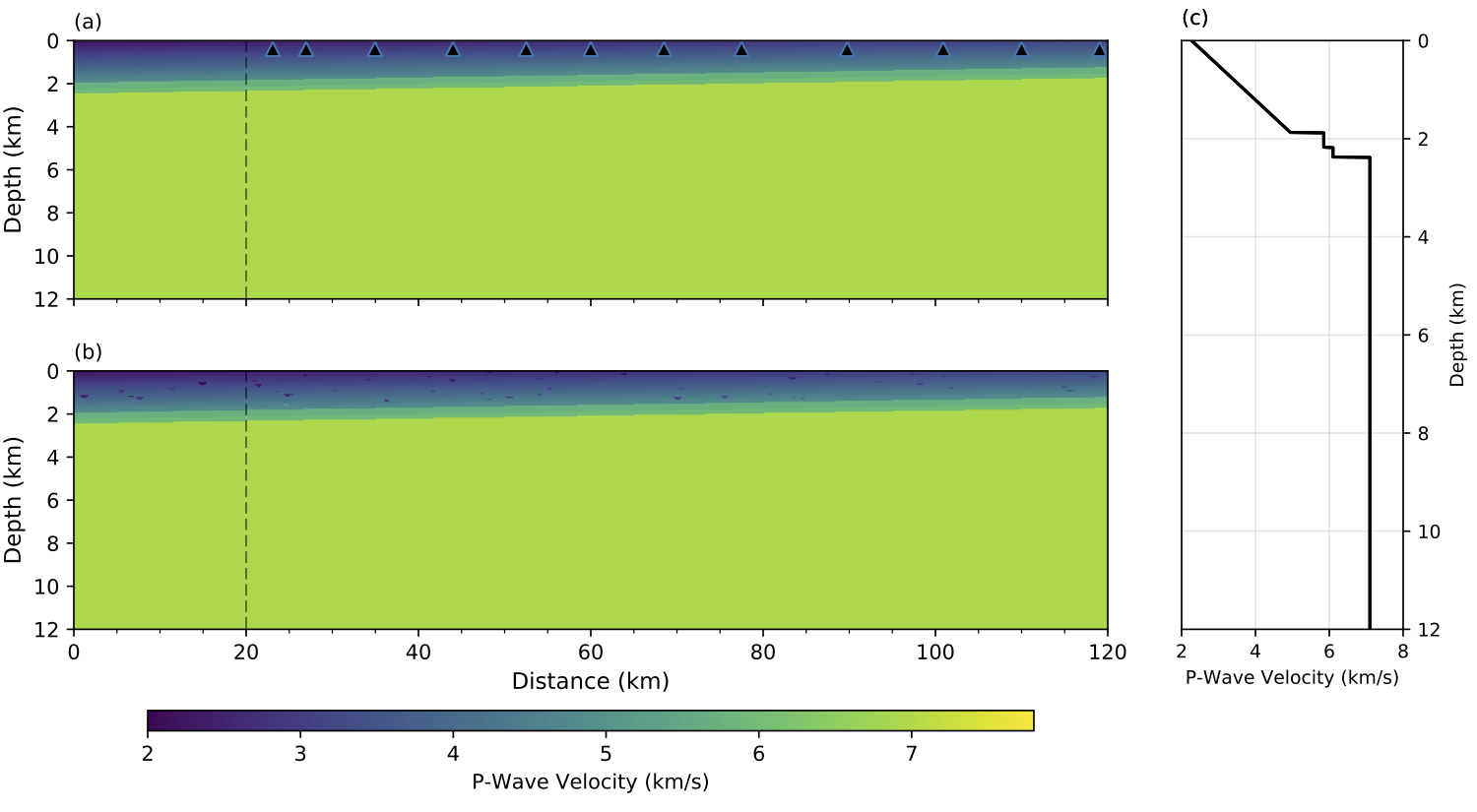
Figure S6. Two velocity models with the synthetic seismographs as triangles. (a) The homogeneous velocity model with a gradient zone (VP 2.1 km/s, ∆VP 1.43 km/s/km) in the top layer, overlaying the Dolomite limestone (Arbuckle group; 5.58 km/s). This marine stratigraphy overlays the granitic basement, which is modeled with a weathering layer (6.1 km/s) on top of the granite (7.1 km/s). (b) The compositional heterogeneous model’s gradient layer is interrupted by paleochannels filled with fluvial sandstones as negative velocity anomalies. (c) A 1D profile of the velocity model at a distance of 20 km (dashed line).
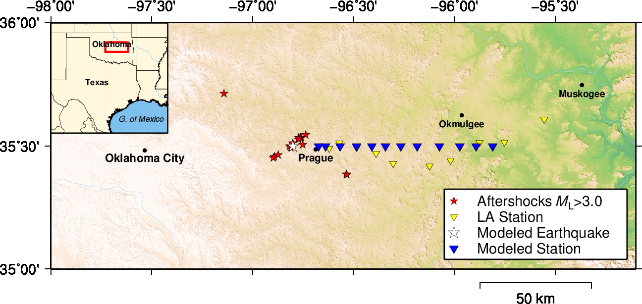
Figure S7. Map showing the locations of the modeled earthquake (white star) and seismometers (blue triangles) relative to the installed seismographs (yellow triangles) and epicenters of the relocated aftershocks (red stars).
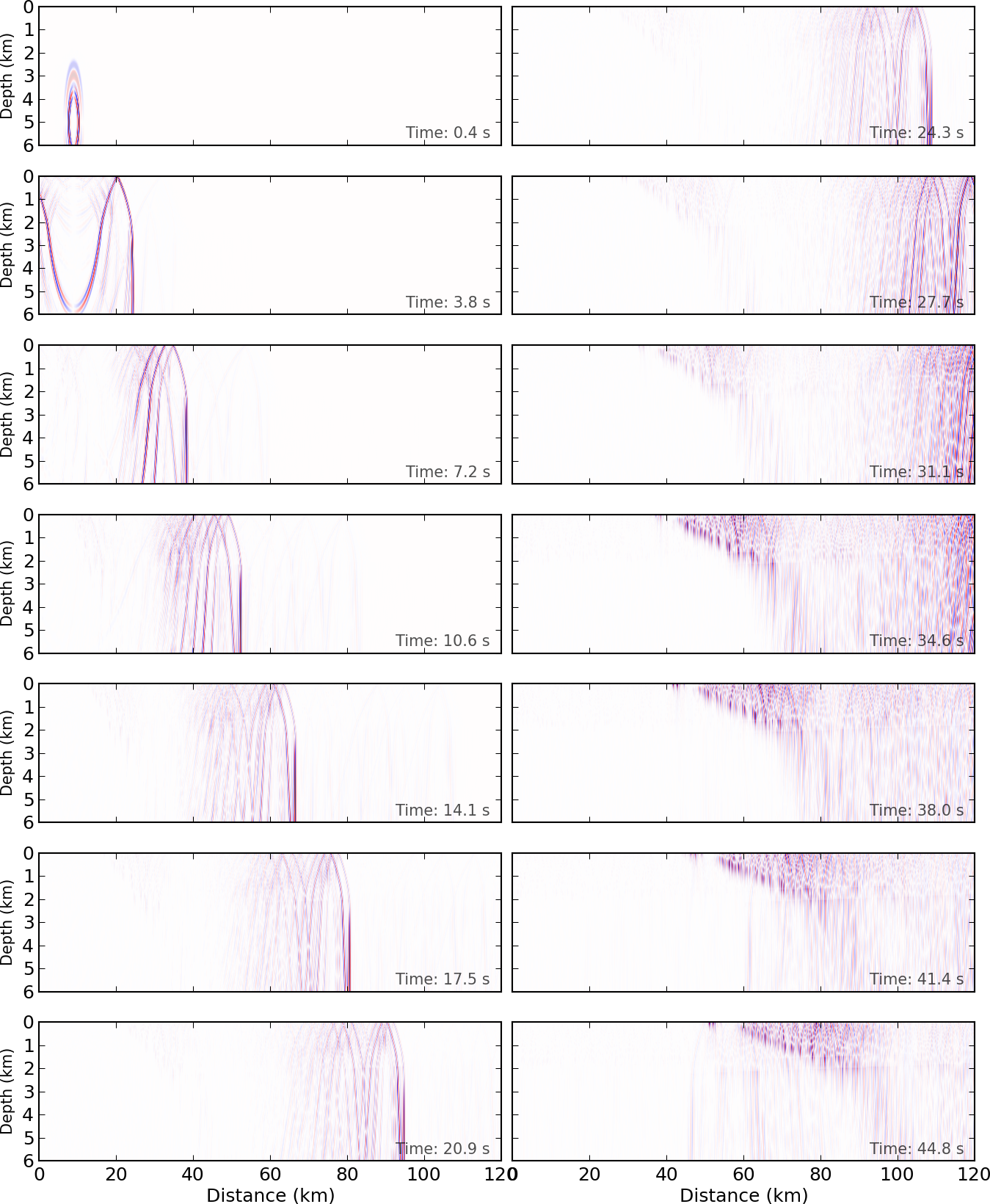
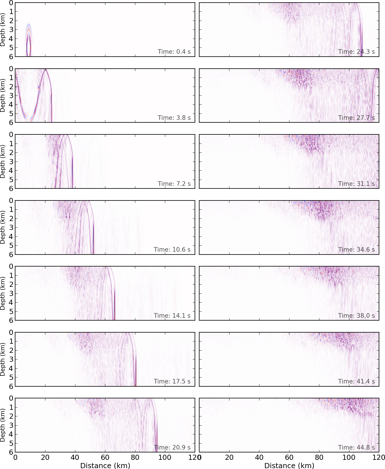
Figure S8. Propagation of the wavefield in the homogeneous gradient model from a source at 5.0 km depth. The development of numerous S-wave multiples can be seen within the first 30 s of the model’s run time, as moving arches of wavefronts. The low energy wavetrain that becomes visible at 31 s was not absorbed by the left damping boundary of the model.
Figure S9. Propagation of the wavefield from a source at 5.0 km focal depth in the heterogeneous model. An unstrucutured S-wave energy packet develops from the direct S waves and disperses after ~3 s into the model’s run time; subsequently this strong S-wave coda spatially expands as it follows the direct S wave with slower velocities.
Seismic data were provided by Incorporated Research Institutions for Seismology (IRIS) and U.S. Geological Survey (USGS) Pasadena. The ZQ network data were recorded by IRIS Rapid Array Mobilization Program (RAMP) and are publicly available through the IRIS Data Management Center (http://www.iris.edu/, last accessed August 2015). The large aperture (LA) network was a temporary network installed by the USGS Pasadena. See Table S1 for detailed configuration.
Joseph, L. (1986). Subsurface analysis, “Cherokee” Group (Des Monesian), portions of Lincoln, Pottawatomie, Seminole, and Okfuskee counties, Oklahoma, The Shale Shaker 12, 44–69.
[ Back ]