This electronic supplement consists of six figures and two tables. Figure S1 describes the hypocentral distances sampled at each station of the studied data set for the main event of the 20 May 2012 Ferrara seismic sequence, whereas Figures S2–S5 describe the moment tensor (MT) solutions that were obtained using three different velocity models. Velocity models are all described in Table S1: the global model ak135 (Kennett et al., 1995), similar to what used by Pondrelli et al. (2012), the Venetian Plains (Vuan et al., 2011), and the Central Italy, Apennines, model (CIA; Herrmann et al., 2011). Table S2 provides the focal parameters of the main event that occurred on 20 May 2012, as we obtain them with the different velocity models. The bottom entry in Table S2 (Padania) is from Malagnini et al. (2012).
For the Venetian Plains model, we show the MT solutions obtained using two different bandwidths, because the bandwidth indicated by Saraò and Peruzza (2012) caused a strong ringing of the transverse components of most synthetic seismograms, as shown in Figure S5. Figure S6 describes the site terms from the ground-motion regression.
Table S1. Parameters of different velocity models.
Table S2. MT solutions for the mainshock of 20 May 2012 at 02:03:53.00, latitude 44.89° and longitude 11.23°. Table indicates the model used in the MT inversion, the three angles of strike, dip, rake, the moment magnitude Mw, the centroid depth, the range of periods used in this study, and the root mean square (rms) misfit.
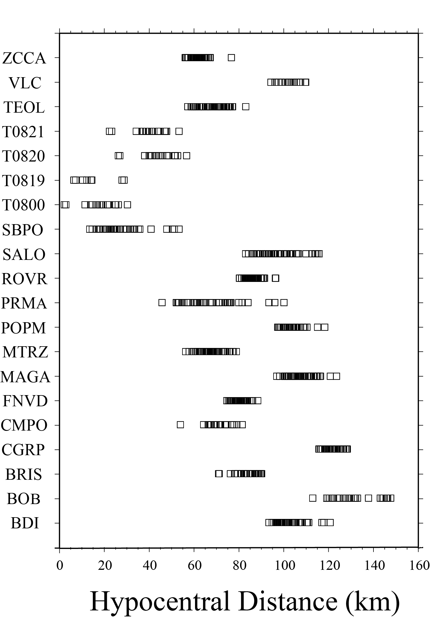
Figure S1. Our data set of hypocentral distances. Names starting with a “T” followed by a sequence of four numbers indicate temporary stations deployed within hours after the mainshock of 20 May 2012. Based on the recommendation published by Malagnini and Dreger (2016), the distribution shown in this figure is less than optimal. Nevertheless, stable results could be obtained for all the events used in this study.
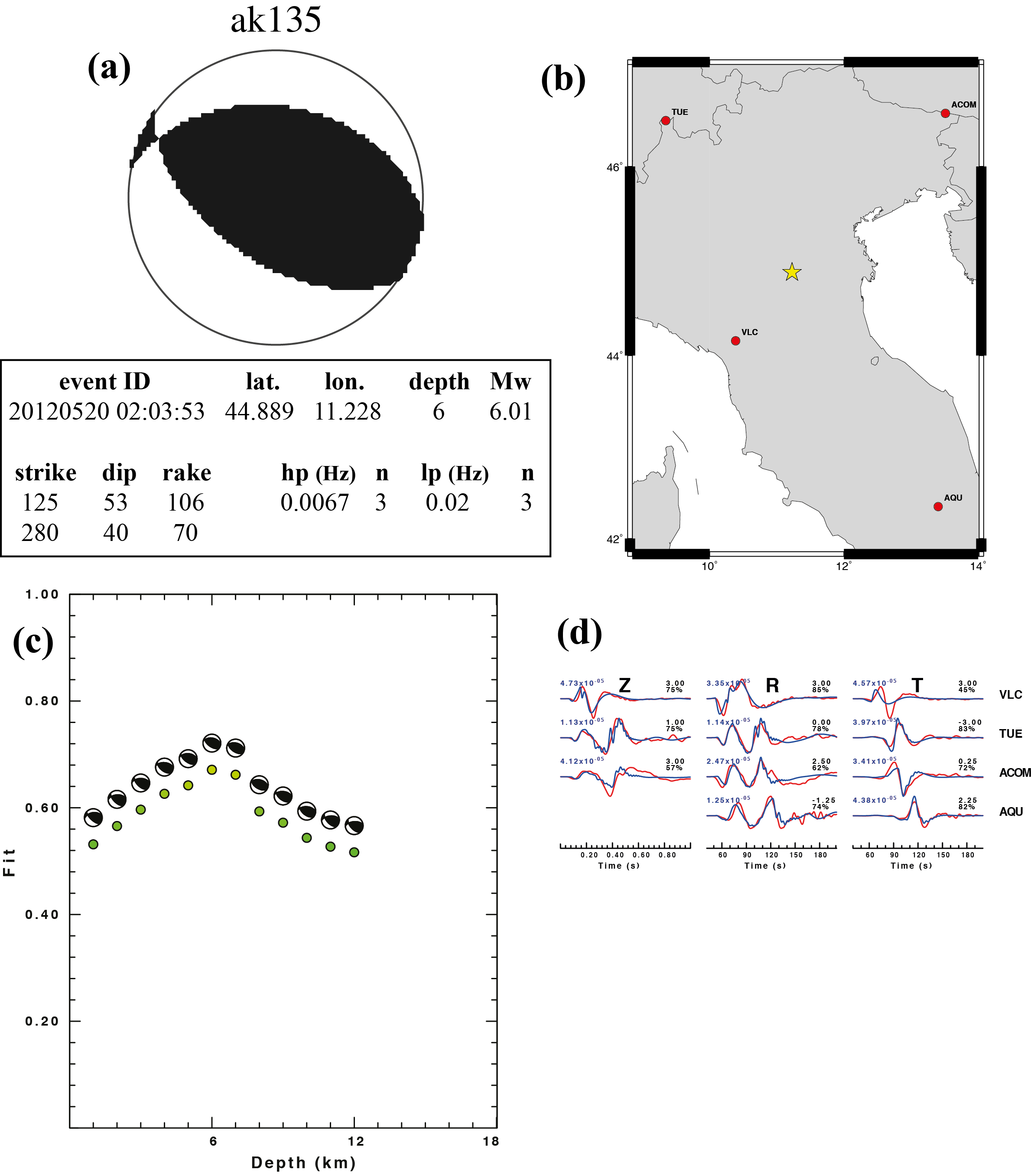
Figure S2. The MT solution computed with ak135 model by Kennett et al. (1995; in the 0.0067–0.02 Hz frequency range). (a) The focal mechanism plot, with the indication of all the geometric parameters, the origin time, the epicentral coordinates, and the parameters used to band-pass filter the waveforms; (b) the map of the station distribution, with the epicentral location of the specific event; (c) the plot of fit versus centroid depth (green dots), with the corresponding focal mechanisms; and (d) all the recorded waveforms that went through the inversion procedure (red), each one with the corresponding synthetic seismogram from the best-fit MT (blue). For each couple of seismograms, we indicate the maximum amplitude of the observed waveform (in blue), the percentage of fit, and the time shift, in seconds, of the synthetic with respect to the observed seismogram used to maximize the best fit.
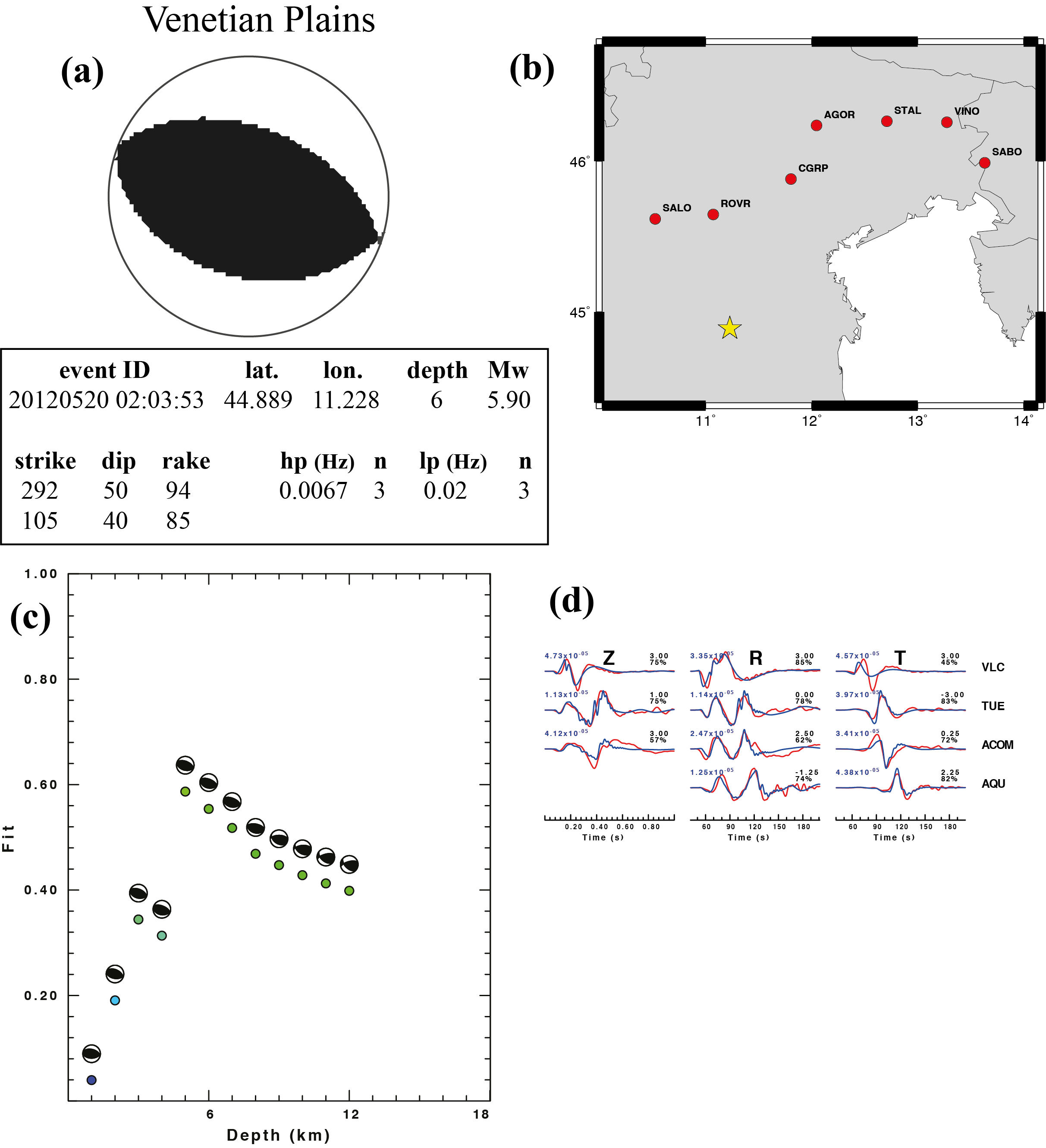
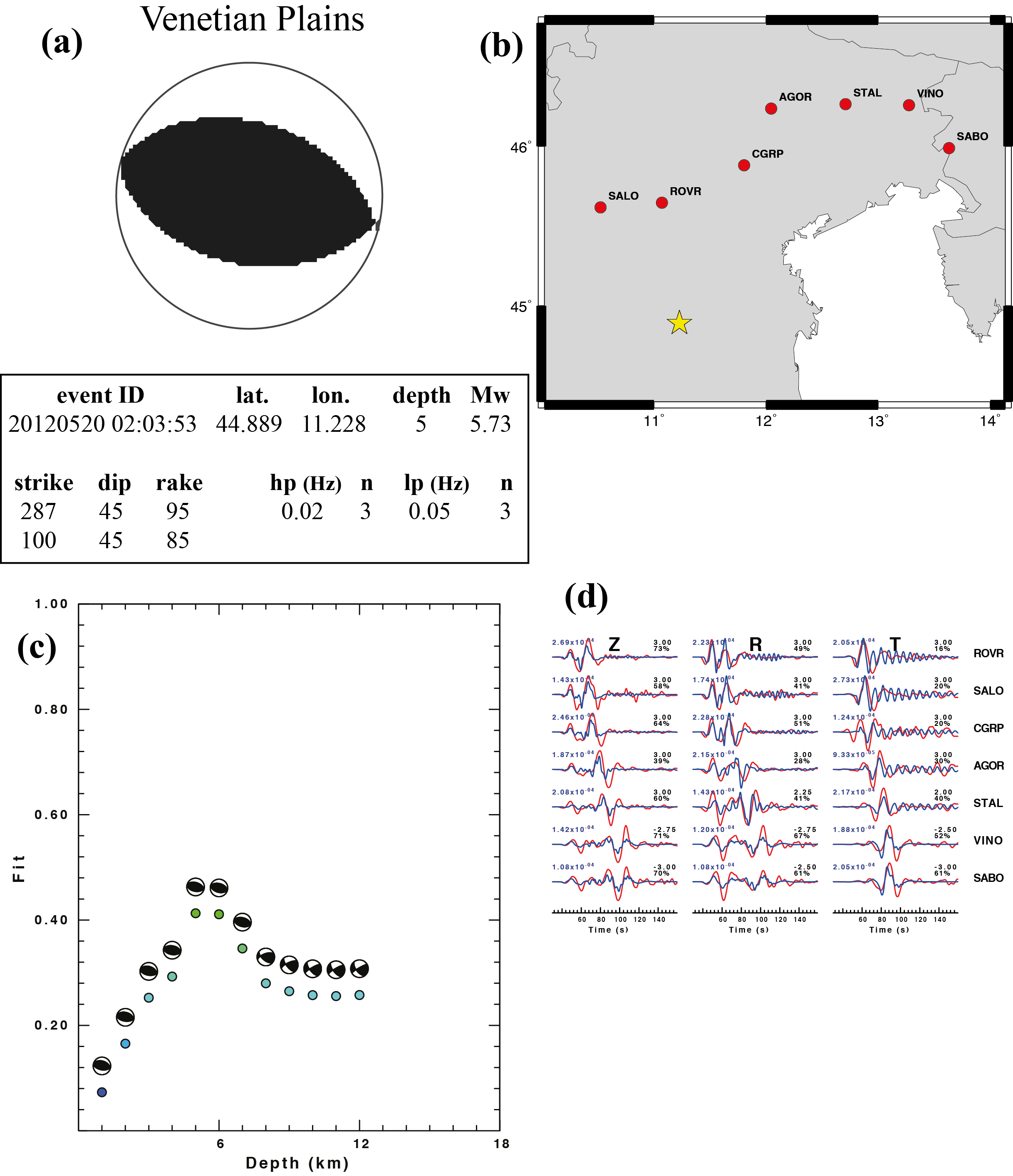
Figure S3. The MT solution computed with Venetian Plains model by Vuan et al. (2011; in the 0.0067–0.02 Hz frequency range). (a) The focal mechanism plot, with the indication of all the geometric parameters, the origin time, the epicentral coordinates, and the parameters used to band-pass filter the waveforms; (b) the map of the station distribution, with the epicentral location of the specific event; (c) the plot of fit versus centroid depth (green dots), with the corresponding focal mechanisms; and (d) all the recorded waveforms that went through the inversion procedure (red), each one with the corresponding synthetic seismogram from the best-fit MT (blue).
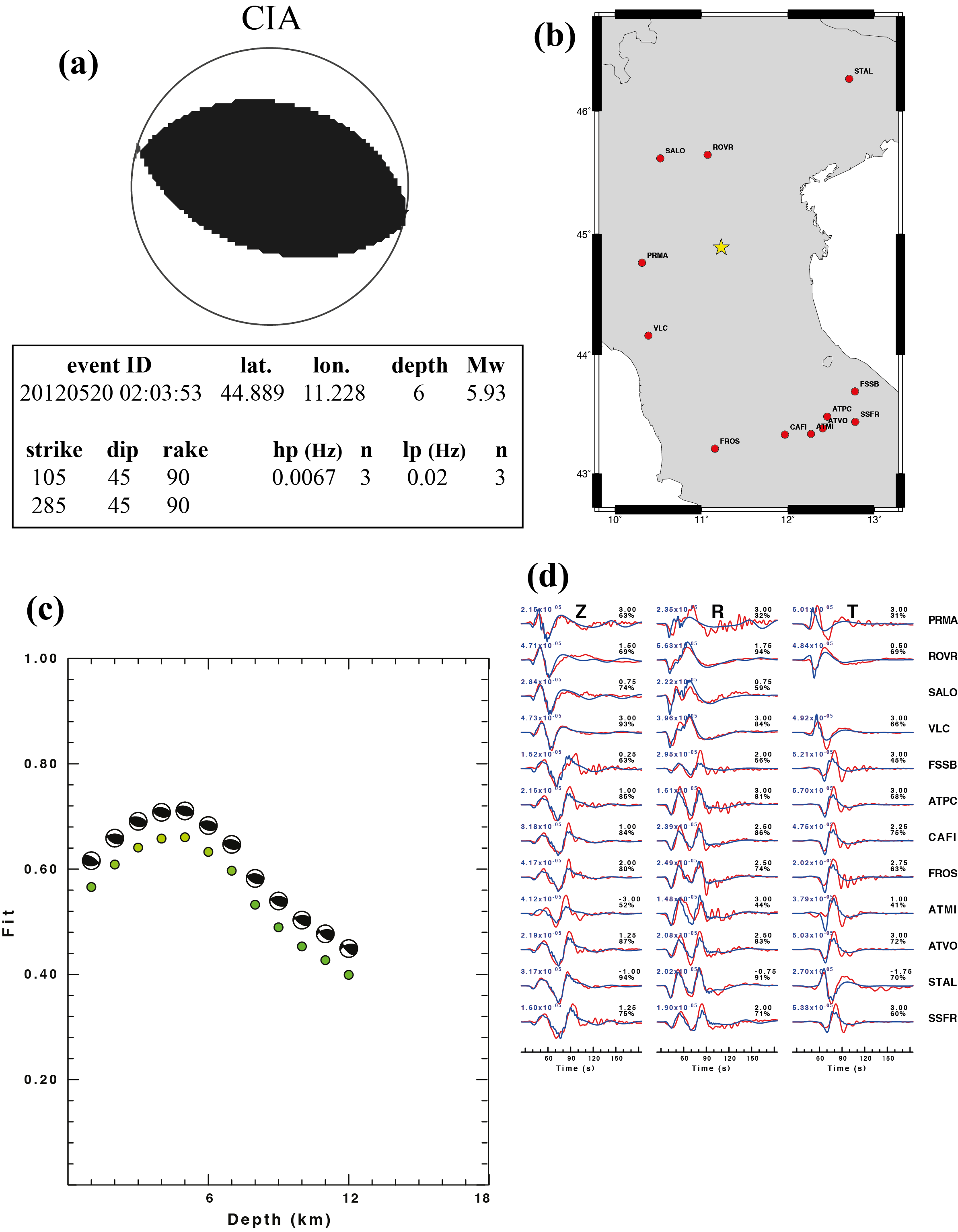
Figure S4. The MT solution computed with the CIA model by Herrmann et al. (2011; in the 0.0067–0.02 Hz frequency range). (a) The focal mechanism plot, with the indication of all the geometric parameters, the origin time, the epicentral coordinates, and the parameters used to band-pass filter the waveforms; (b) the map of the station distribution, with the epicentral location of the specific event; (c) the plot of fit versus centroid depth (green dots), with the corresponding focal mechanisms; and (d) all the recorded waveforms that went through the inversion procedure (red), each one with the corresponding synthetic seismogram from the best-fit MT (blue).
Figure S5. The MT solution computed with Venetian Plains model by Vuan et al. (2011; in the 0.02–0.05 Hz frequency range, that was used by Saraò and Peruzza, 2012). (a) The focal mechanism plot, with the indication of all the geometric parameters, the origin time, the epicentral coordinates, and the parameters used to band-pass filter the waveforms; (b) the map of the station distribution, with the epicentral location of the specific event; (c) the plot of fit versus centroid depth (green dots), with the corresponding focal mechanisms; and (d) all the recorded waveforms that went through the inversion procedure (red), each one with the corresponding synthetic seismogram from the best-fit MT (blue). See the ringing on the transverse components of the synthetic seismograms on most stations (all, except VINO and SABO) and the consequent misfit.
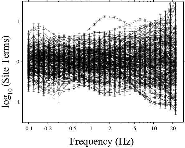
Figure S6. Site terms from the regressions of the ground motions. Each term in this figure represents an anomaly with respect to the average horizontal site term calculated on the stations SALO, MAGA, and ROVR.
Herrmann, R. B., L. Malagnini, and I. Munafo’ (2011). Regional moment tensors of the 2009 L’Aquila earthquake sequence, Bull. Seismol. Soc. Am. 101, no. 3, 975–993, doi: 10.1785/0120100184.
Kennett, B. L. N., E. R. Engdahl, and R. Buland (1995). Constraints on seismic velocities in the earth from travel times, Geophys. J. Int. 122, 108–124.
Malagnini, L., and D. S. Dreger (2016). Generalized free-surface effect and random vibration theory: A new tool for computing moment magnitudes of small earthquakes using borehole data, Geophys. J. Int. 206, doi: 10.1093/gji/ggw113.
Malagnini, L., R. B. Herrmann, I. Munafò, M. Buttinelli, M. Anselmi, A. Akinci, and E. Boschi (2012). The 2012 Ferrara seismic sequence: Regional crustal structure, earthquake sources, and seismic hazard, Geophys. Res. Lett. 39, L19302, doi: 10.1029/2012GL053214.
Pondrelli, S., S. Salimbeni, P. Perfetti, and P. Danecek (2012). Quick regional centroid moment tensor solutions for the Emilia 2012 (northern Italy) seismic sequence, Ann. Geophys. 55, no. 4, doi: 10.4401/ag-6146.
Saraò, A., and L. Peruzza (2012). Fault-plane solutions from moment-tensor inversion and preliminary Coulomb stress analysis for the Emilia Plain, Ann. Geophys. 55, no. 4, doi: 10.4401/ag-6134.
Vuan, A., P. Klin, G. Laurenzano, and E. Priolo (2011). Far-source long-period displacement response spectra in the Po and Venetian Plains (Italy) from 3D wavefield simulations, Bull. Seismol. Soc. Am. 101, 1055–1072, doi: 10.1785/0120090371.
[ Back ]