This electronic supplement contains figures of histograms of slip and rise time, waveform comparisons between data and synthetics, and slip velocity along the fault plane for a synthetic case as well as for the 2011 7.1 Van, east Turkey, earthquake and the 2010 7.2 El Mayor–Cucapah, Baja California, earthquake.
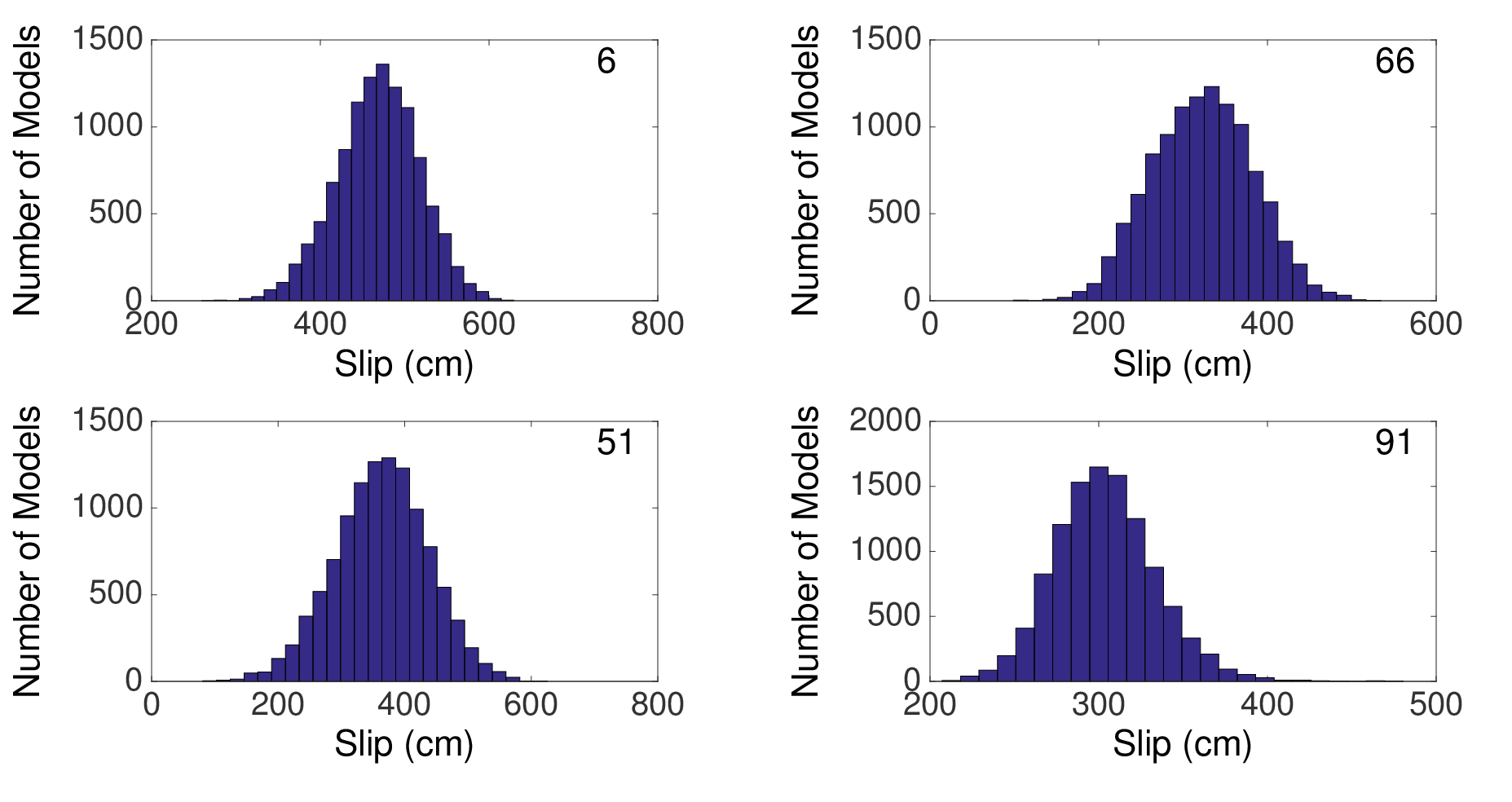
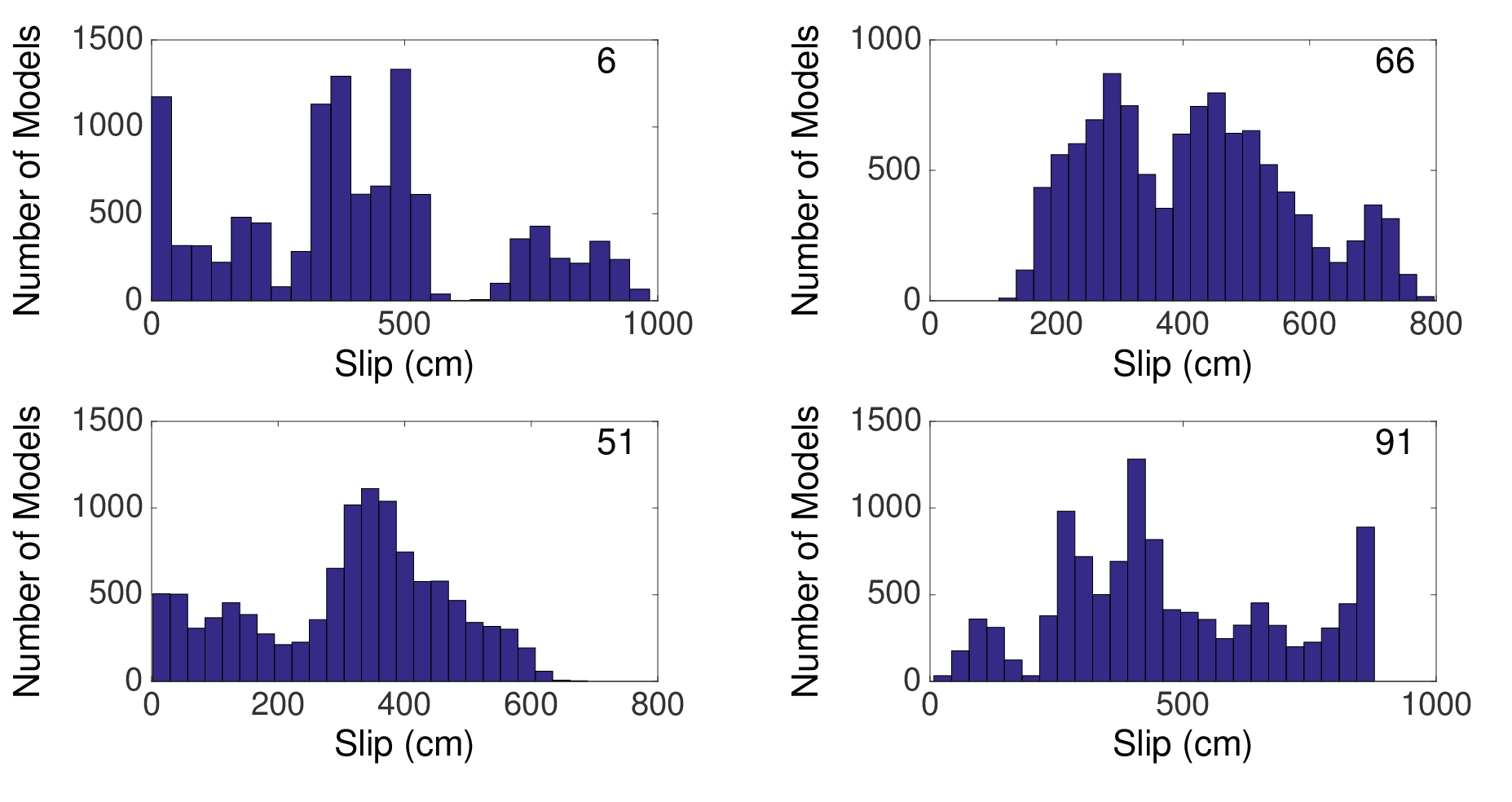
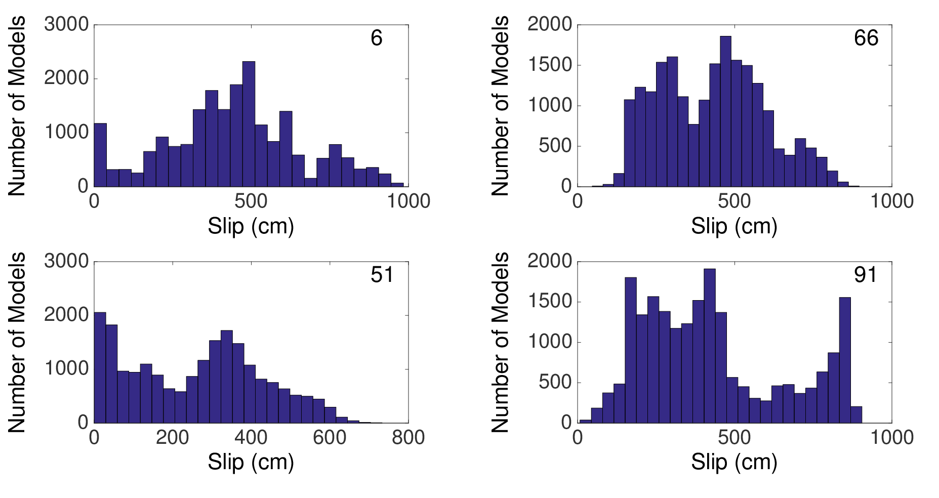
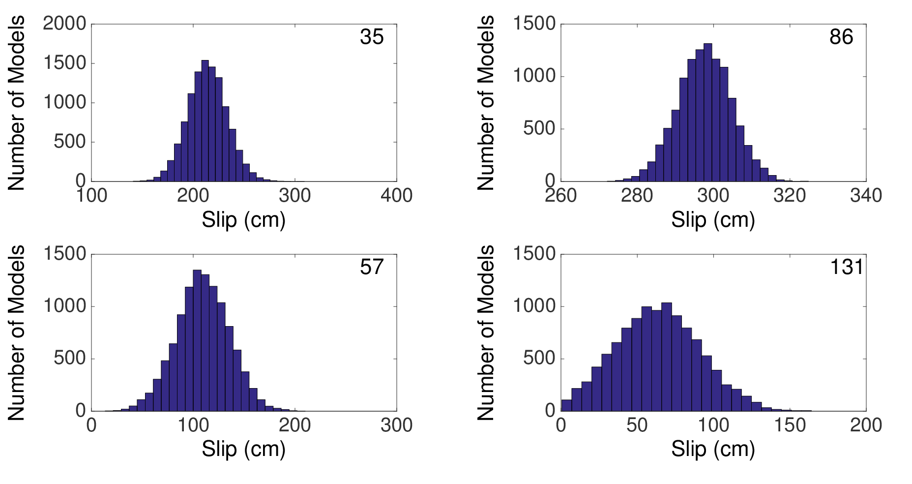
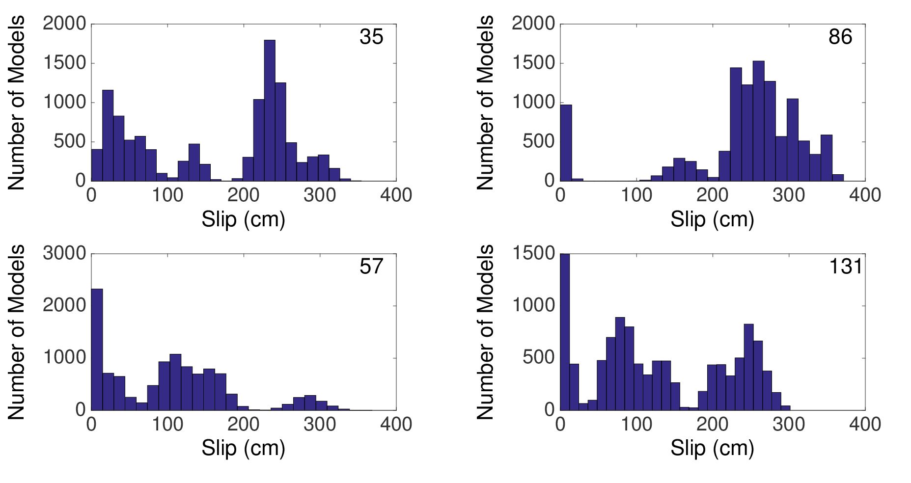
Figure S1. Synthetic scenario histograms of slip for four subfaults (subfault number corresponding to probability density function (PDF) is shown in upper right corner of each graph) for the solution containing (a) a single velocity model, (b) 11 velocity models, and (c) 21 velocity models.
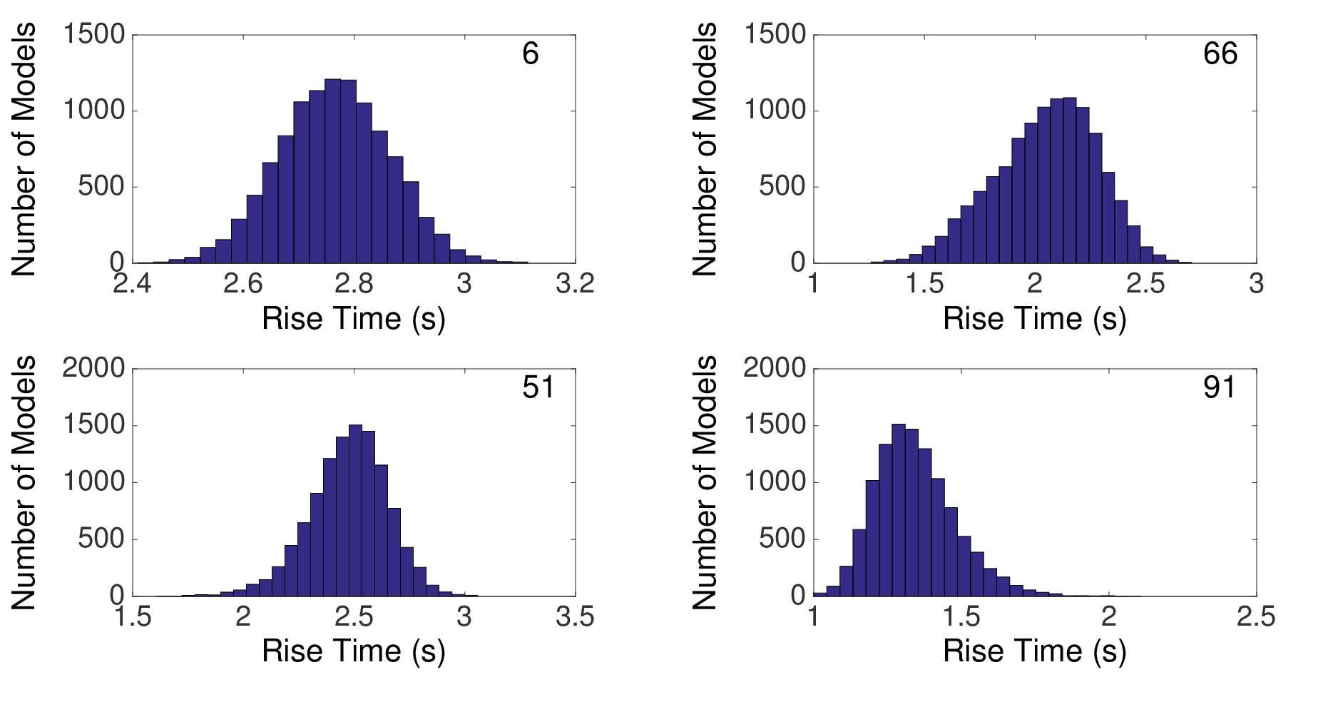
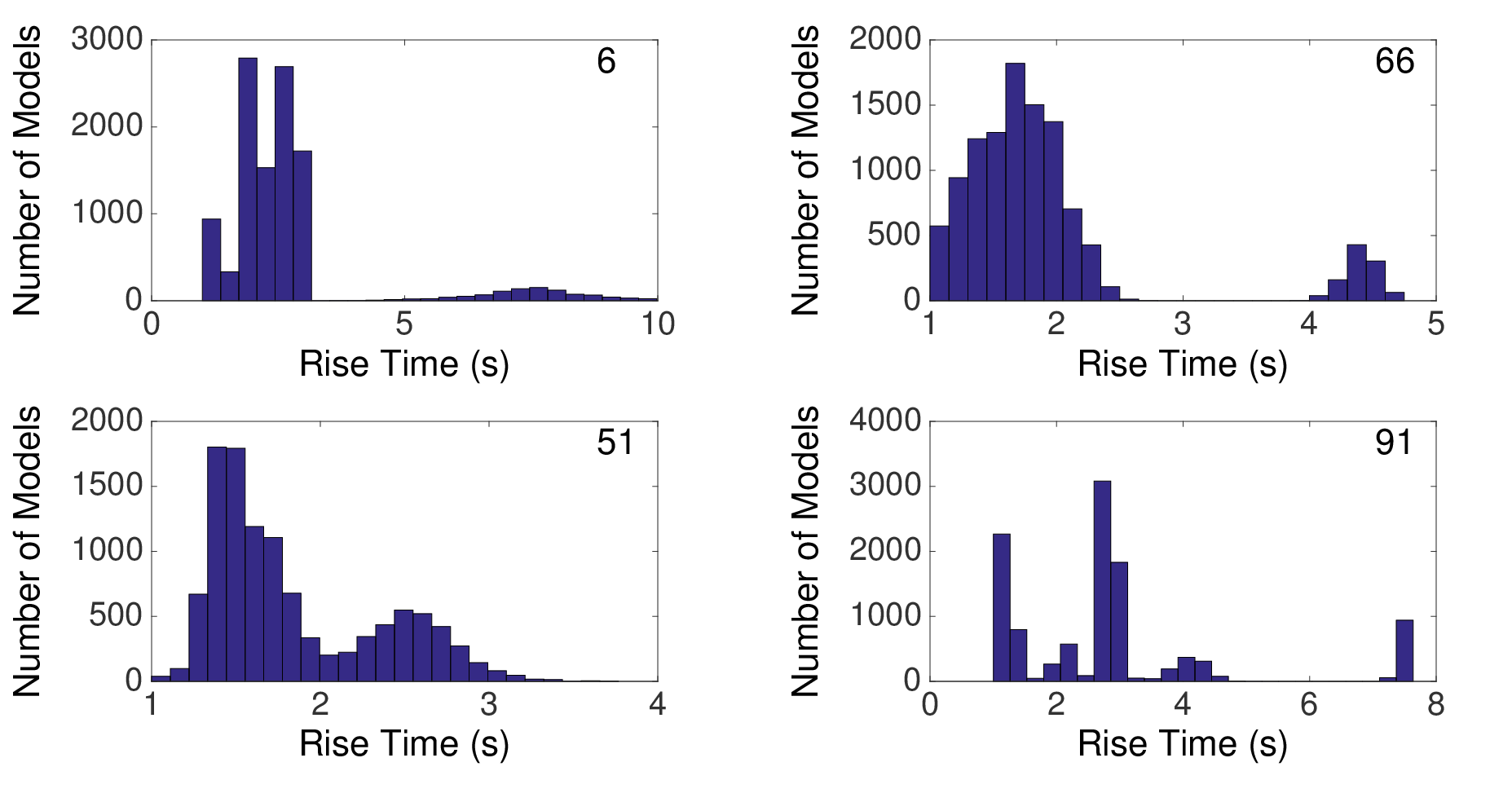
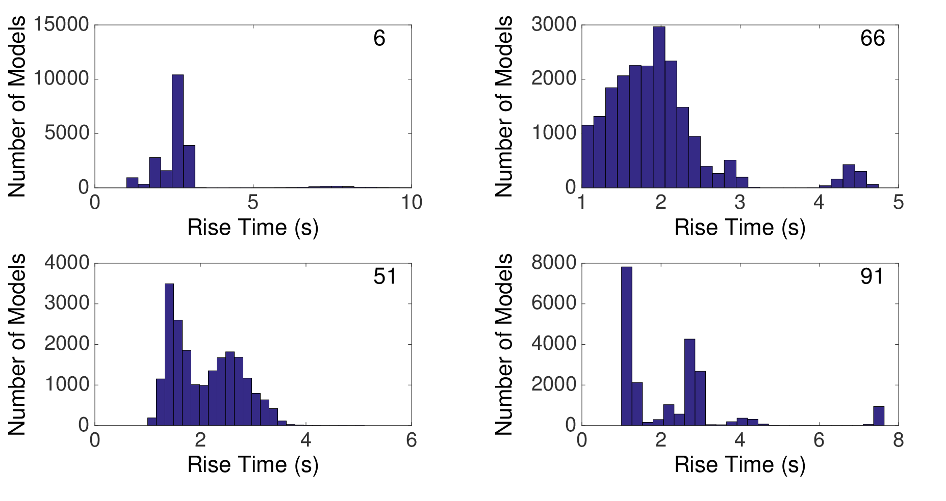
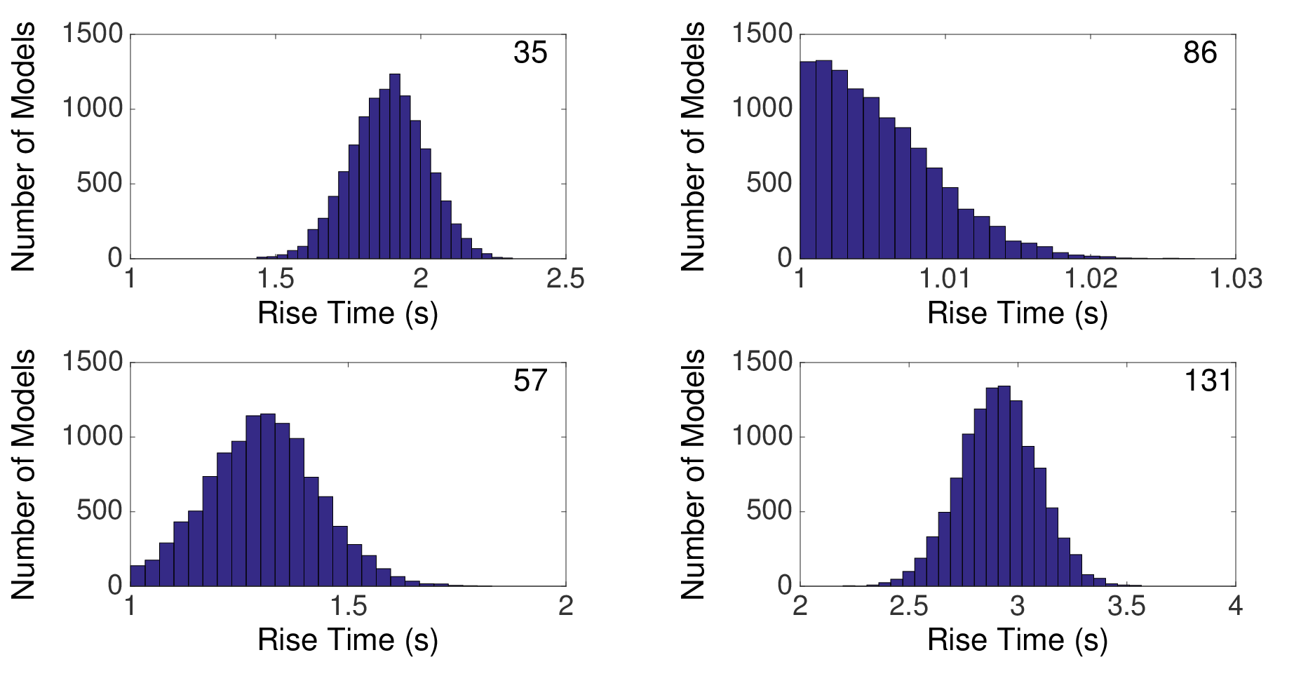
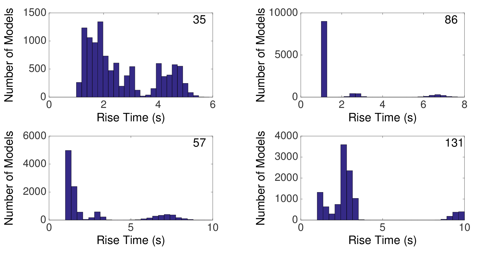
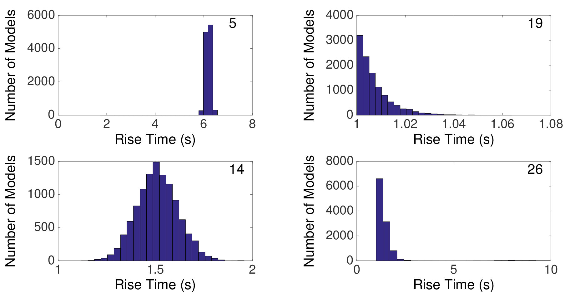
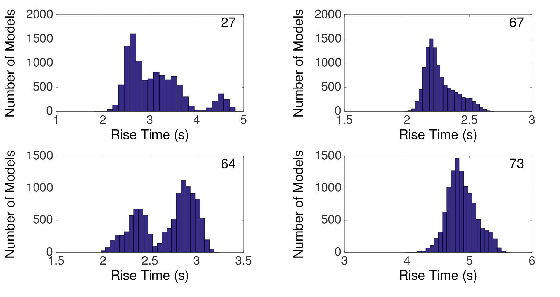
Figure S2. Synthetic scenario histograms of rise times for four subfaults for the solution containing (a) a single velocity model, (b) 11 velocity models, and (c) 21 velocity models.
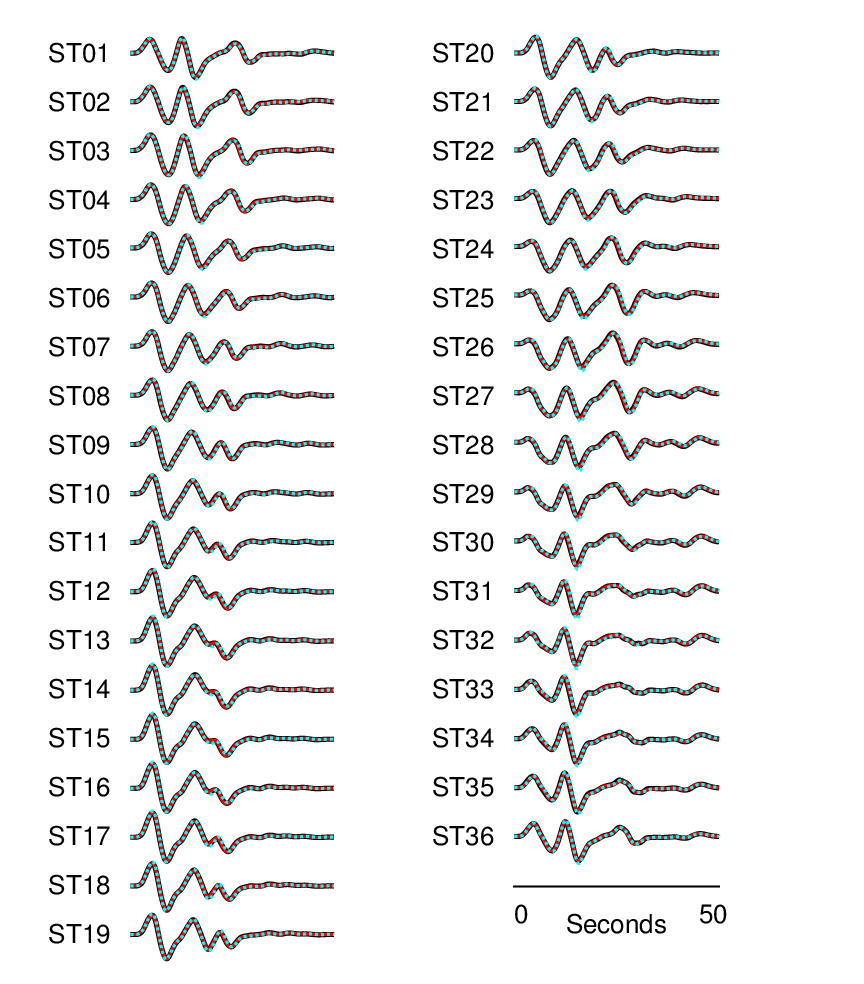
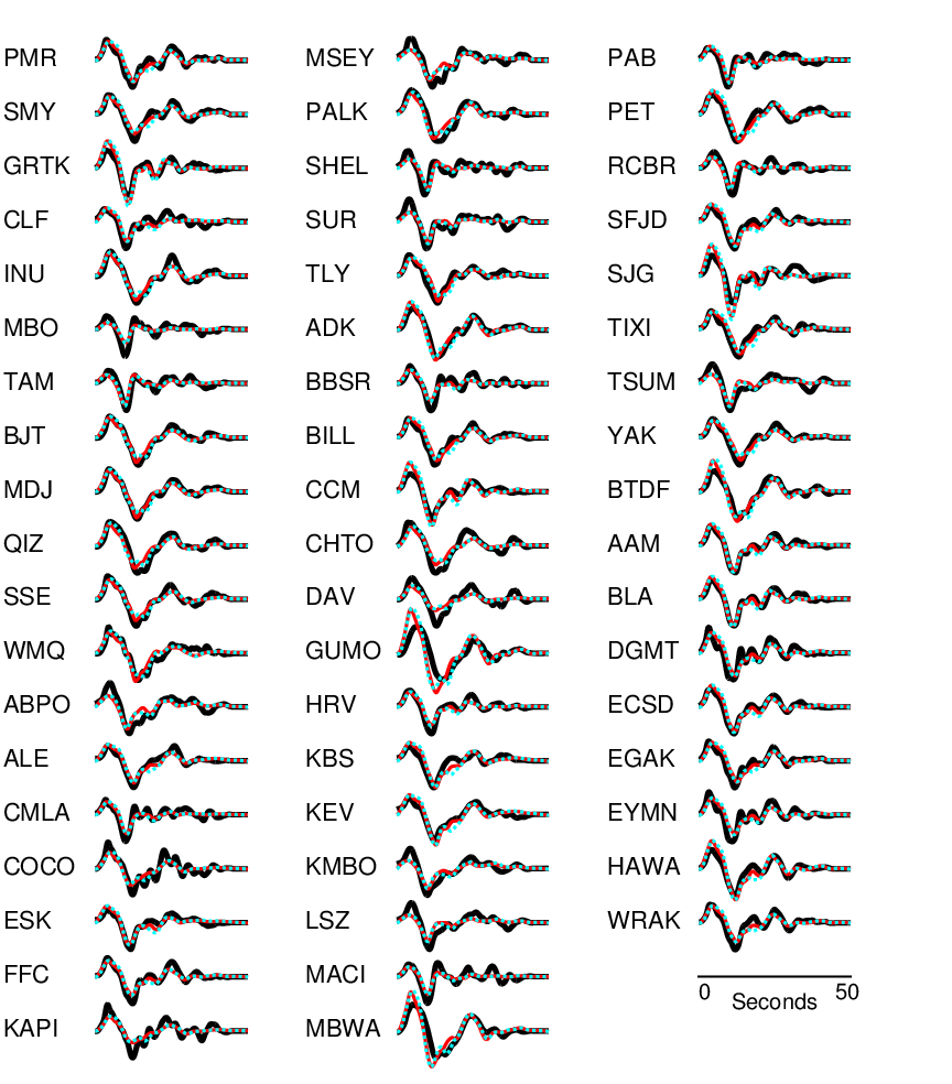
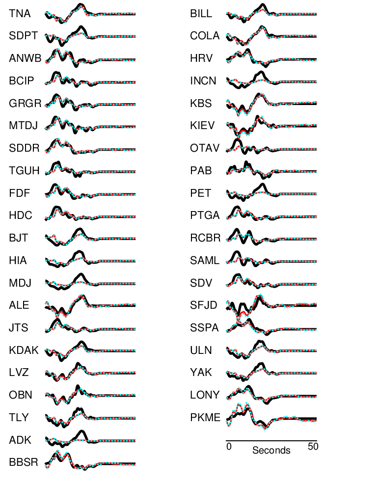
Figure S3. Observed teleseismic P waveforms of the synthetic model (thick black line), predicted data for the single velocity model solution (red), and a 10 velocity models solution (blue dashed line) for the synthetic scenario using a 50-s record length.
Figure S4. Histograms of slip for four subfaults for the 2011 Van earthquake for the solution containing (a) a single velocity model and (b) 11 velocity models.
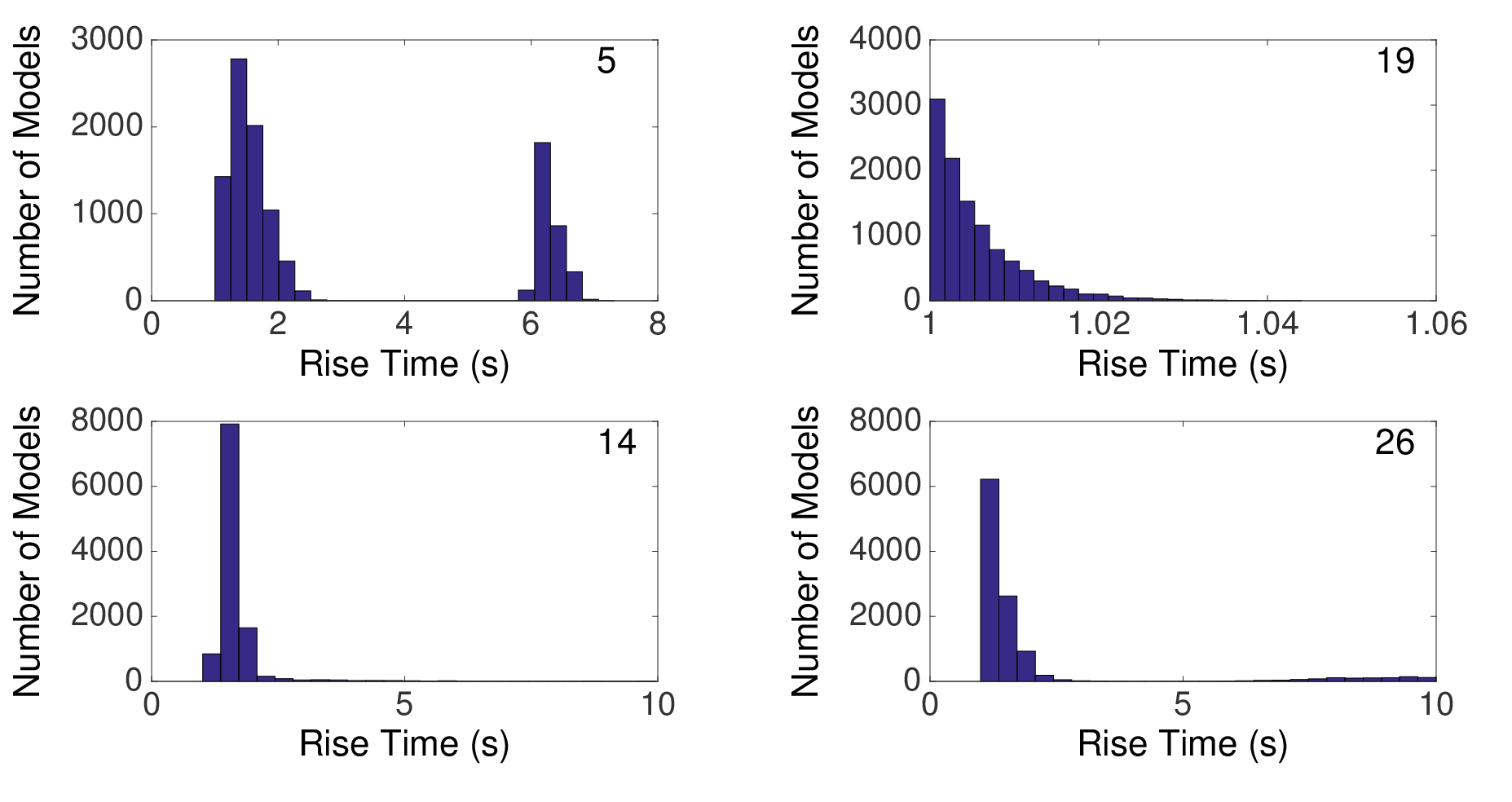
Figure S5. Histograms of rise time for four subfaults for the 2011 Van earthquake for the solution containing (a) a single velocity model and (b) 11 velocity models.
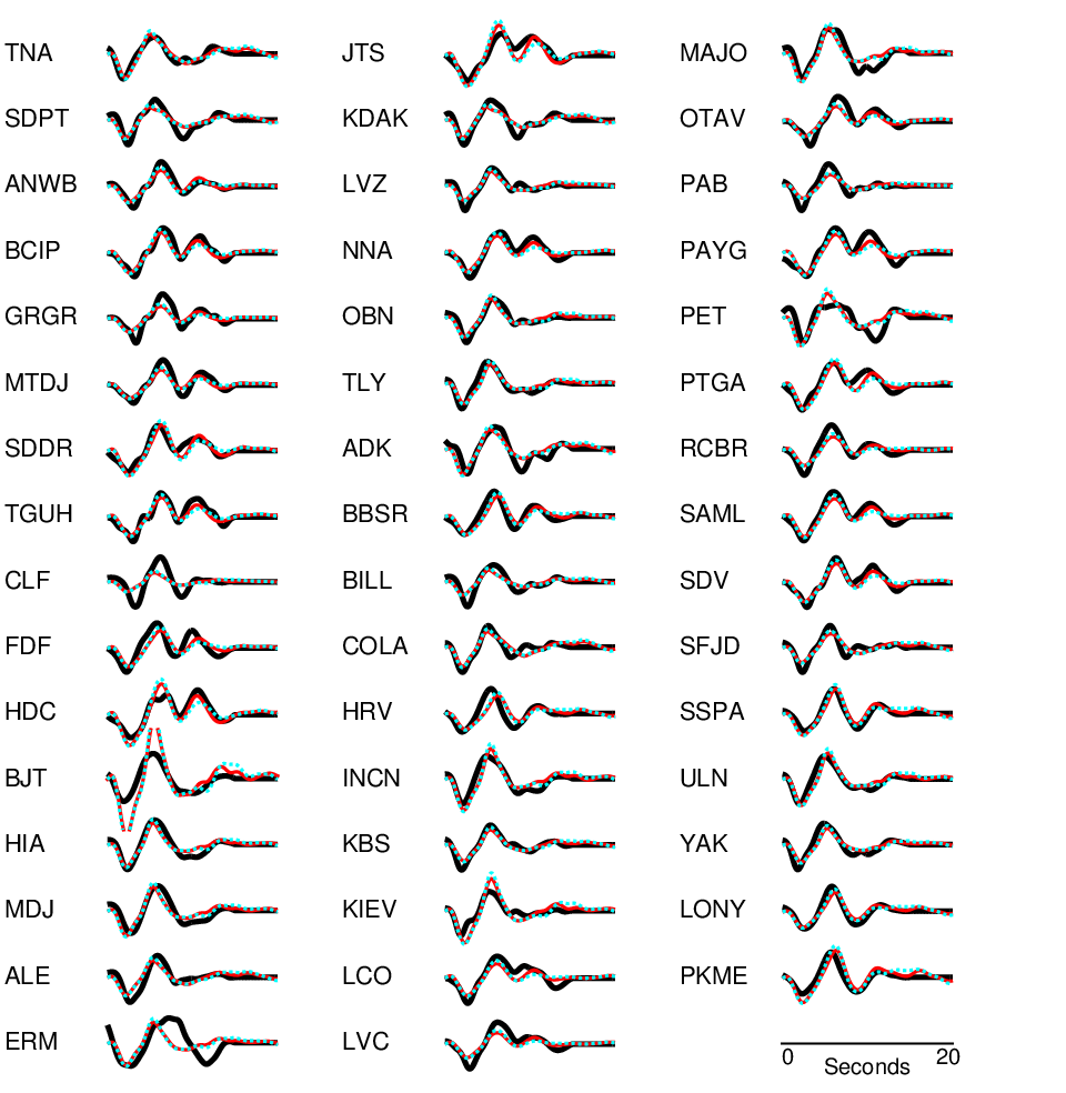
Figure S6. Observed (thick black line) and predicted teleseismic P waveforms for the single velocity model solution (red) and 11 velocity models solution (blue dashed line) for the 2011 Van earthquake using a 50-s record length.
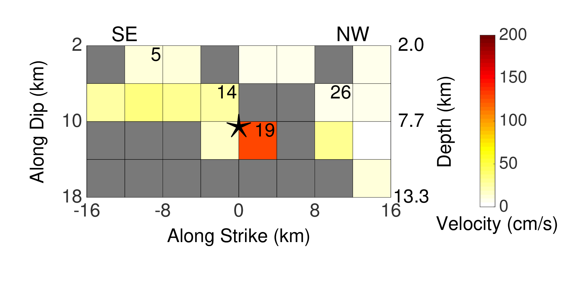
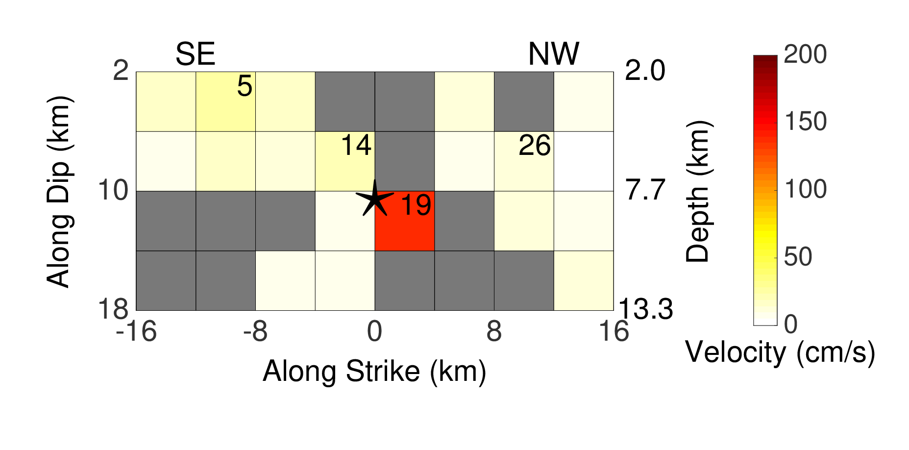
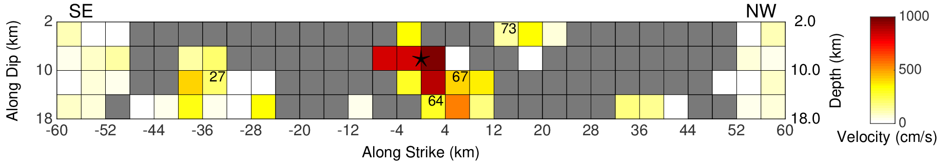
Figure S7. Slip velocity distributions for the subevent of the 2010 El Mayor–Cucapah, Baja California, earthquake: (a) distribution with a single velocity model and an angle constrain of is applied from the inferred rake, and (b) distribution when using multiple velocity models throughout the inversion process with the angle constraint applied. Numbered subfaults are explored further. Subfaults shown in gray correspond to slip values that are 20 cm or less.
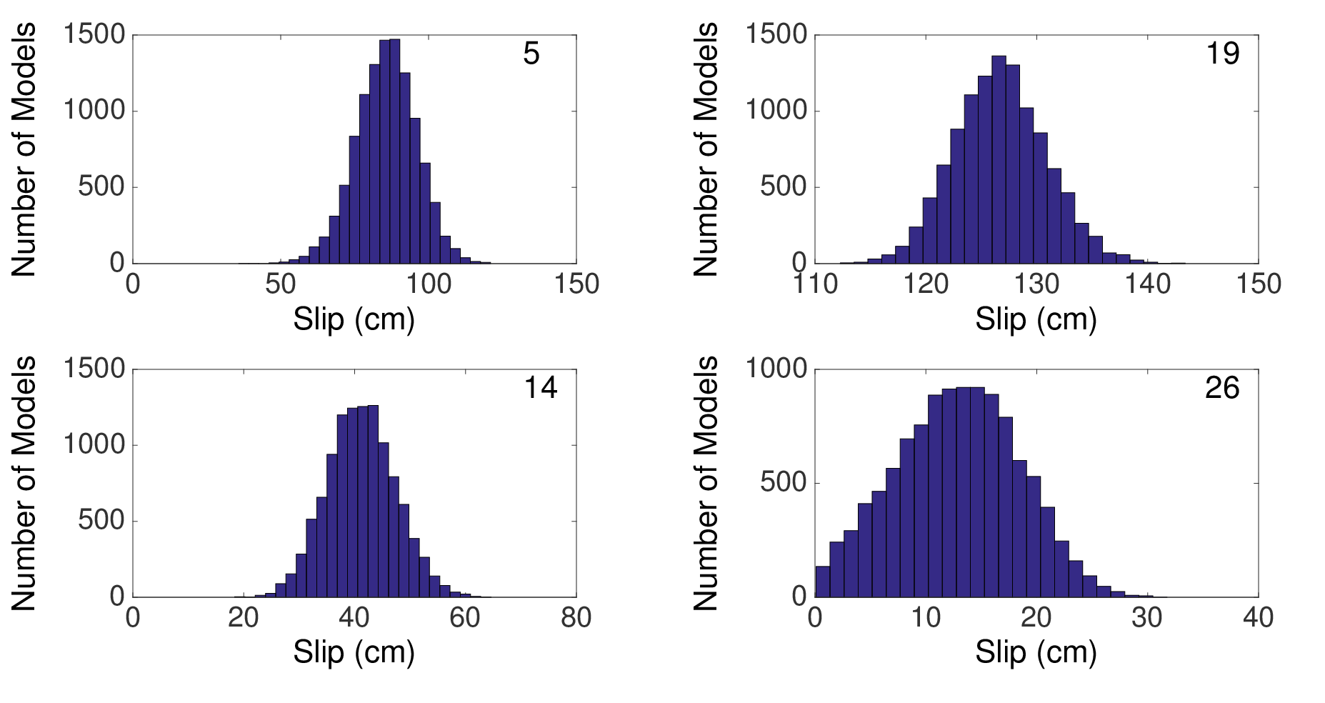
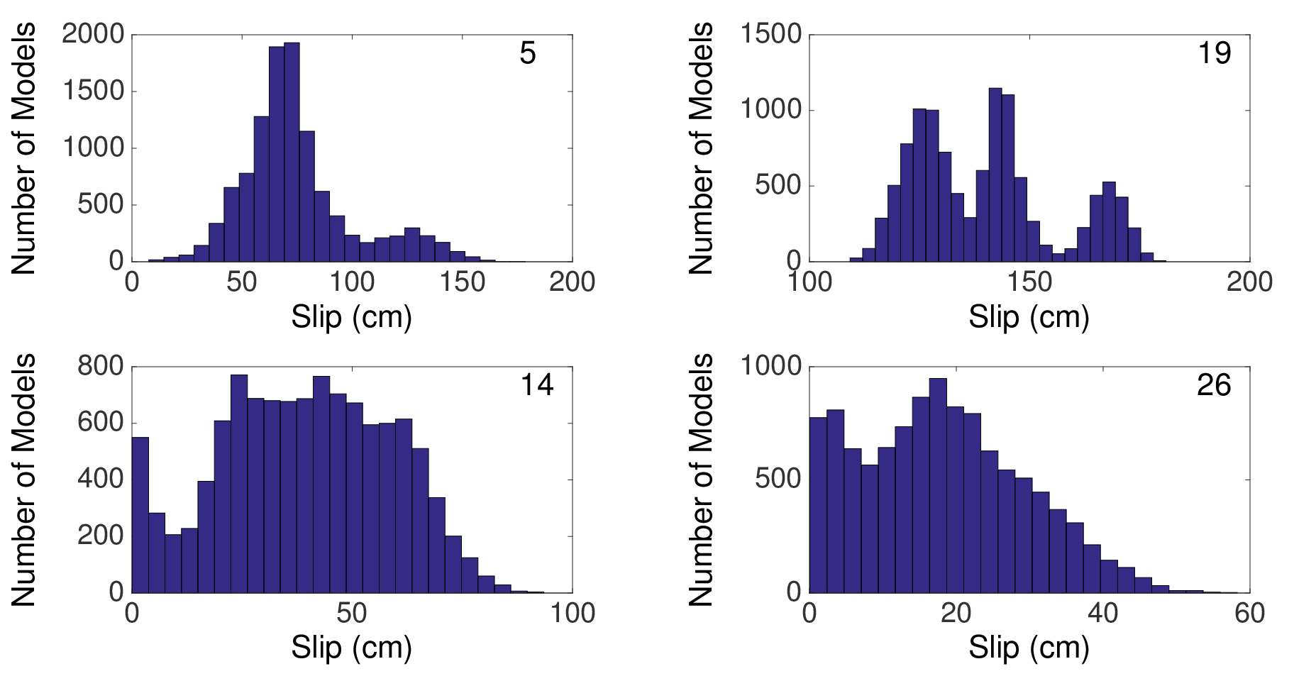
Figure S8. Histograms of slip for four subfaults for the subevent of the 2010 El Mayor–Cucapah earthquake for the solution containing (a) a single velocity model and (b) 11 velocity models.
Figure S9. Histograms of rise time for four subfaults for the subevent of the 2010 El Mayor–Cucapah earthquake for the solution containing (a) a single velocity model and (b) 11 velocity models.
Figure S10. Observed (thick black line) and predicted teleseismic P waveforms for the single velocity model solution (red) and 11 velocity models solution in (blue dashed line) for the subevent of the 2010 El Mayor–Cucapah earthquake using a 20-s record length.
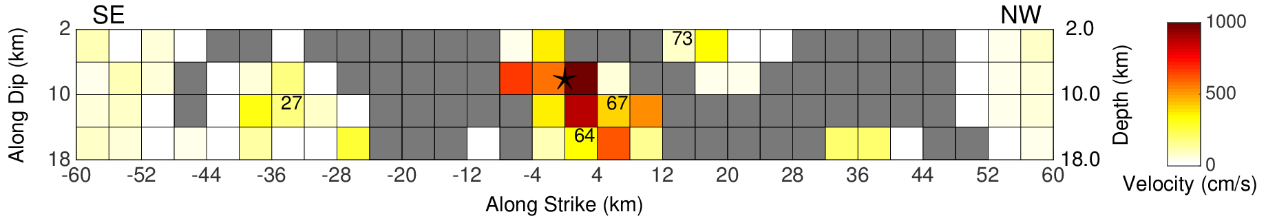
Figure S11. Slip velocity distributions for the main event of the 2010 El Mayor–Cucapah, Baja California, earthquake: (a) distribution with a single velocity model and an angle constraint of applied from the inferred rake, and (b) distribution when using multiple velocity models throughout the inversion process with the angle constraint applied. Numbered subfaults are further explored. Subfaults shown in gray correspond to slip values that are 20 cm or less.
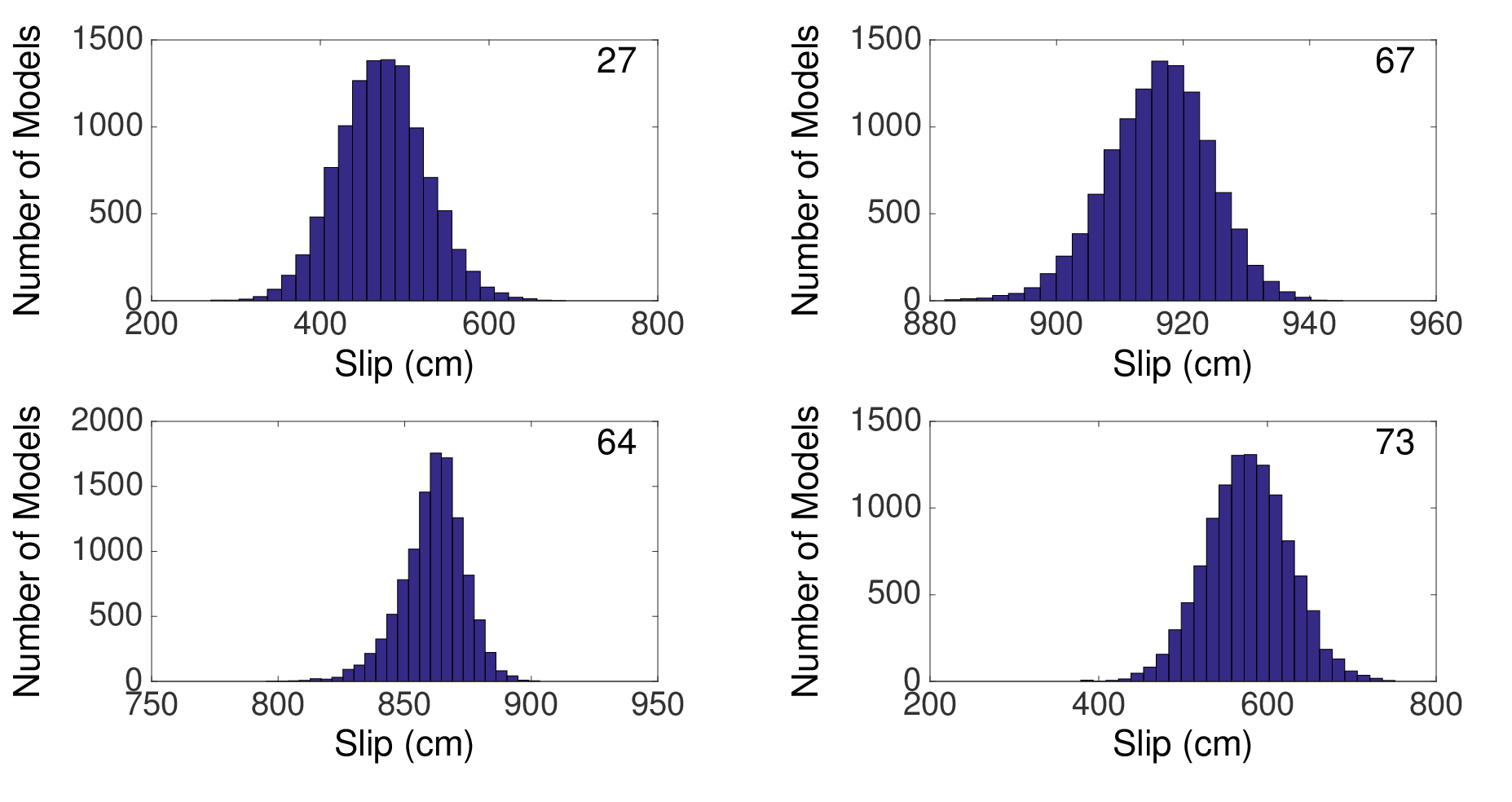
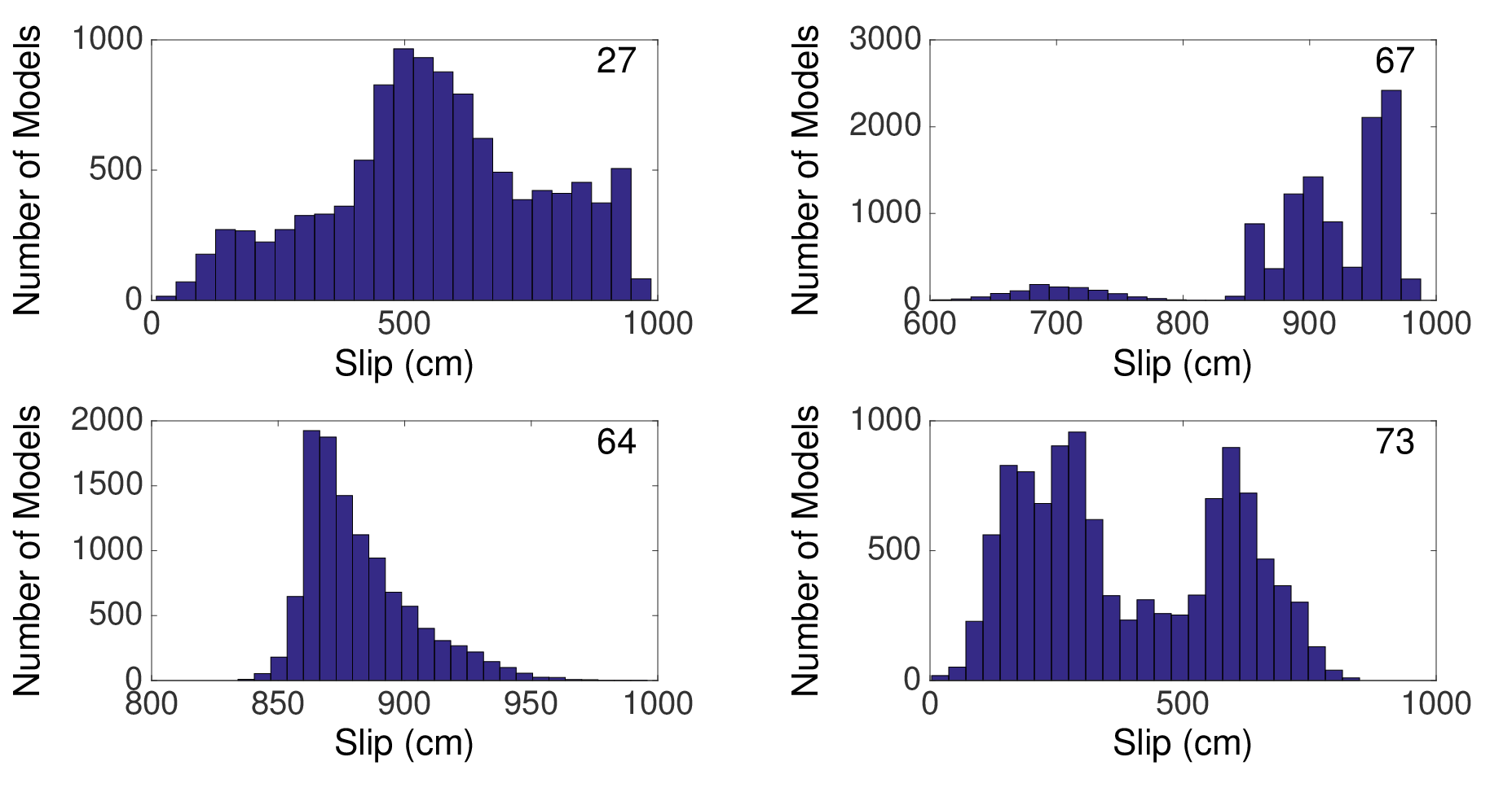
Figure S12. Histograms for slip for four subfaults for the main event of the 2010 El Mayor–Cucapah earthquake for the solution containing (a) a single velocity model and (b) 11 velocity models.
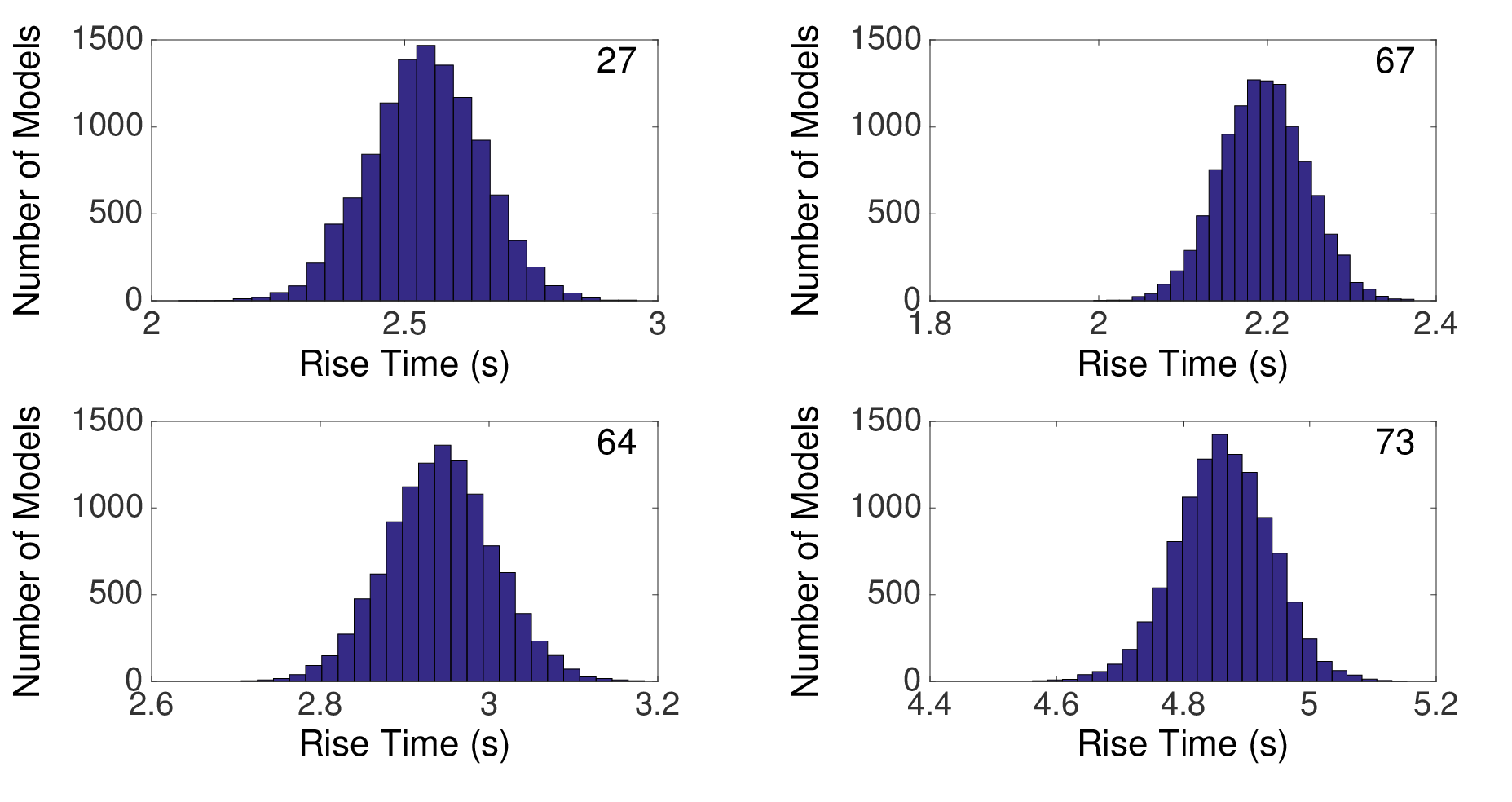
Figure S13. Histograms for rise time for four subfaults for the main event of the 2010 El Mayor–Cucapah earthquake for the solution containing (a) a single velocity model and (b) 11 velocity models.
Figure S14. Observed (thick black line) and predicted teleseismic P waveforms for the single velocity model solution (red) and 11 velocity models solution (blue dashed line) for the main event of the 2010 El Mayor–Cucapah earthquake using a 50-s record length.
[ Back ]