This electronic supplement contains the methods and figures of relocated aftershocks, interferograms, residuals, transformations, and seismic station locations.
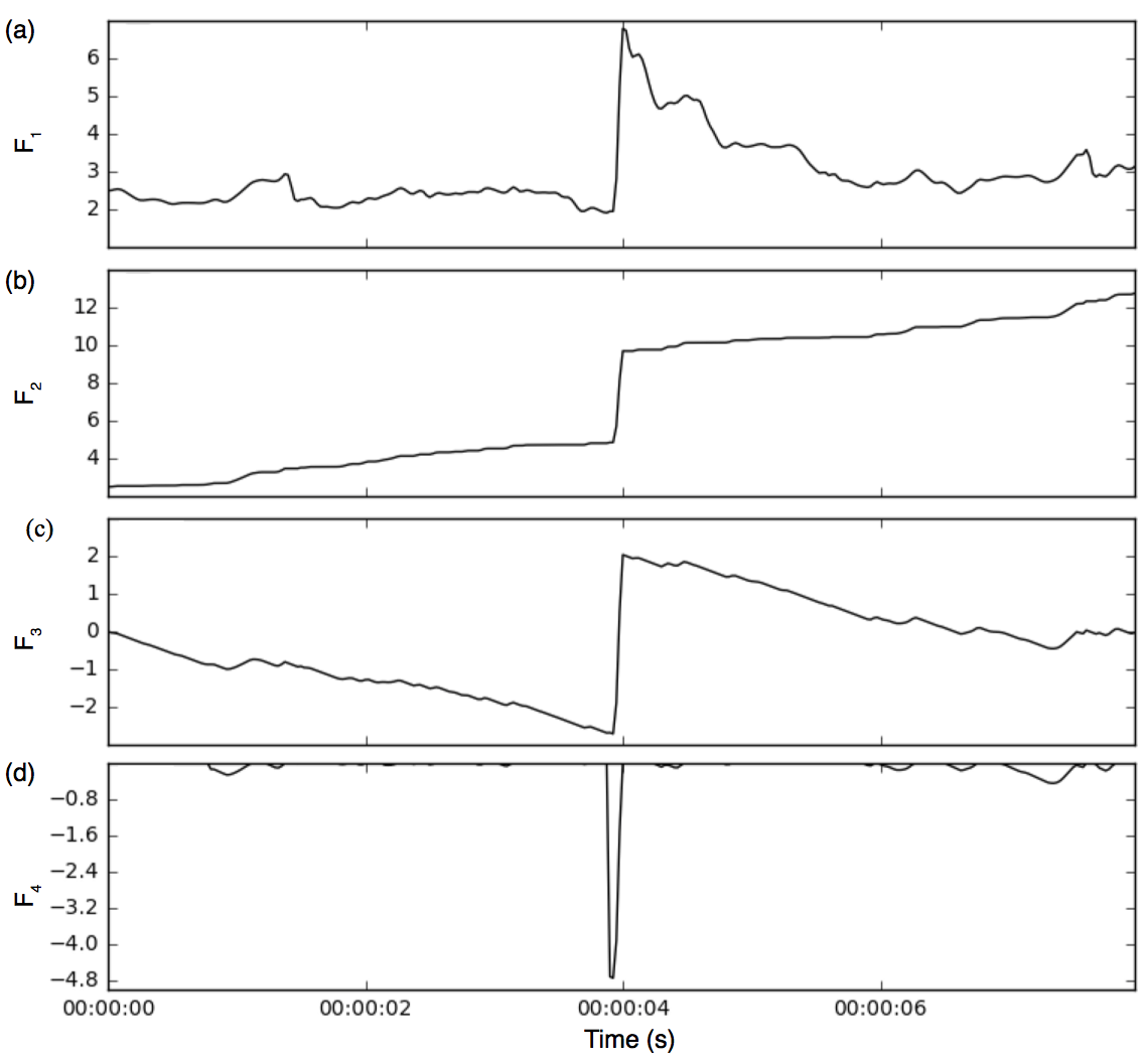
The kurtosis detector implemented for this study was based on the design of the automatic kurtosis-based picker of Baillard et al. (2014). Kurtosis characterizes the shape of the statistical distribution of the seismic data and rapidly increases at the onset time. Consequently, the kurtosis function can be used to detect the onset of a seismic wave. Three transformations are applied to the kurtosis function to obtain a characteristic function from which arrival-time picks can be derived. These transformations remove all strictly negative gradients, remove the linear trend, and scale the amplitudes of the function so that the greatest onset strength corresponds to the greatest minimum of the characteristic function. The kurtosis function and the transform functions can be seen in Figure S4. A 2-s sliding window is moved over the observed station waveform data from which the kurtosis characteristic function is computed.
Results from the kurtosis picker for each station can be seen in Table S1. When selecting picks, both an amplitude threshold and a signal-to-noise ratio (SNR) threshold were used. For all of the picks found in this study, the amplitude threshold was set at 4 and the SNR threshold at 1.5. On average, there were 834 picks selected per day, with the most picks (7029) found on 22 February, the day after the mainshock. The most picks, in total, were selected from station M12A (11,649), the closest station to the mainshock location, and the fewest picks were selected from DUG (568), the farthest station from the mainshock.
Subspace detection is a powerful tool that allows earthquake signals with small amplitude to be detected despite the presence of noise. For each station of interest, the templates used to generate the subspace detector are correlated with the observed data and a sufficient statistic (equivalent to the square of the correlation coefficient) is calculated. Finding the z-score associated with each sufficient statistic evaluates how close (in standard deviations) the current statistic is from the mean sufficient statistic within a considered window. Because the z-score accounts for the changing mean in each considered window, a single cutoff threshold can be selected rather than having to adjust the cutoff for each window. To find a sufficient statistic’s z-score, a Fisher z-transformation is applied to the statistic. The z-transform, given by
is a variance stabilizing and normalizing transformation that results in a practically normal distribution (Fisher, 1921; Fouladi et al., 2002). Using the new approximately normal distribution, a z-score can be found using the mean and standard deviation of the distribution
(Lomax and Hahs-Vaughn, 2013). In this study, detections are declared if the z-score is above 6; that is, the sufficient statistic is at least 6 standard deviations from the mean and the SNR value is 1.5 or higher.
The subspace detections were found using templates that were band-pass filtered at 1–4 Hz with data windows including either P- or S-wave observations. The windowed data ranged in duration from 3 to 25 s for P-wave observations and from 10 to 20 s for S-wave observations. A maximum number of detections of 16,830 (5101 from P templates and 11,729 from S templates) occurred on 22 February, the day following the mainshock. The fewest number of detections was 71 on 23 August, with 10 detections from P templates and 61 detections from S templates. On average, there were 1131 detections per day; there were 370 detections from P templates and 761 detections from S templates. The total number of detections for each station can be seen in Table S1.
HD is a relocation technique that uses Bayesian statistical methods to incorporate a priori arrival-time information when deriving hypocenter confidence ellipsoids (Jordan and Sverdrup, 1981). The HD relocation method finds both relative locations of individual events and the absolute location of the earthquake cluster. The relocation process is an iterative one in two senses. Beyond the iterative aspect of a least-squares inversion to estimate perturbations of starting hypocentral parameters from travel-time residuals, it involves repeated cycles of outlier detection and removal, which we refer to as cleaning. Outlier travel-time readings are determined relative to the spread of the travel-time residuals for each station and phase pair observed multiple times in the dataset. The spread function is insensitive to large outliers (i.e., robust), requires no estimate of central location, and makes no assumptions about the underlying distribution; with samples from a normal distribution, it reduces to an estimate of the standard deviation. Absolute travel-time residuals, relative to the theoretical arrival time, are thus transformed into cluster residuals, relative to the mean of the arrival times and are scaled by the current estimate of spread (empirical reading error). Although the spread function is rather robust against bias by large outliers, the least-squares relocation is not, especially because the data are weighted inversely to the current estimate of empirical reading error. Therefore, the locations (and possibly phase identifications) may change substantially as outliers are removed and the distribution of data weights in the inverse problem is altered by the cleaning process. The threshold above which readings are designated as outliers is large at first; it is gradually reduced, followed at each step by relocation to obtain new starting locations and estimates of empirical reading errors, until the distribution of cluster residuals for each station phase is approximately normal; that is, the estimate of spread is taken as an estimate of sigma, and all readings are within 3σ of the mean for that station phase.
Table S1. The number of P and S picks from the subspace detector (SD) along with the number of picks from the kurtosis detector for each station.
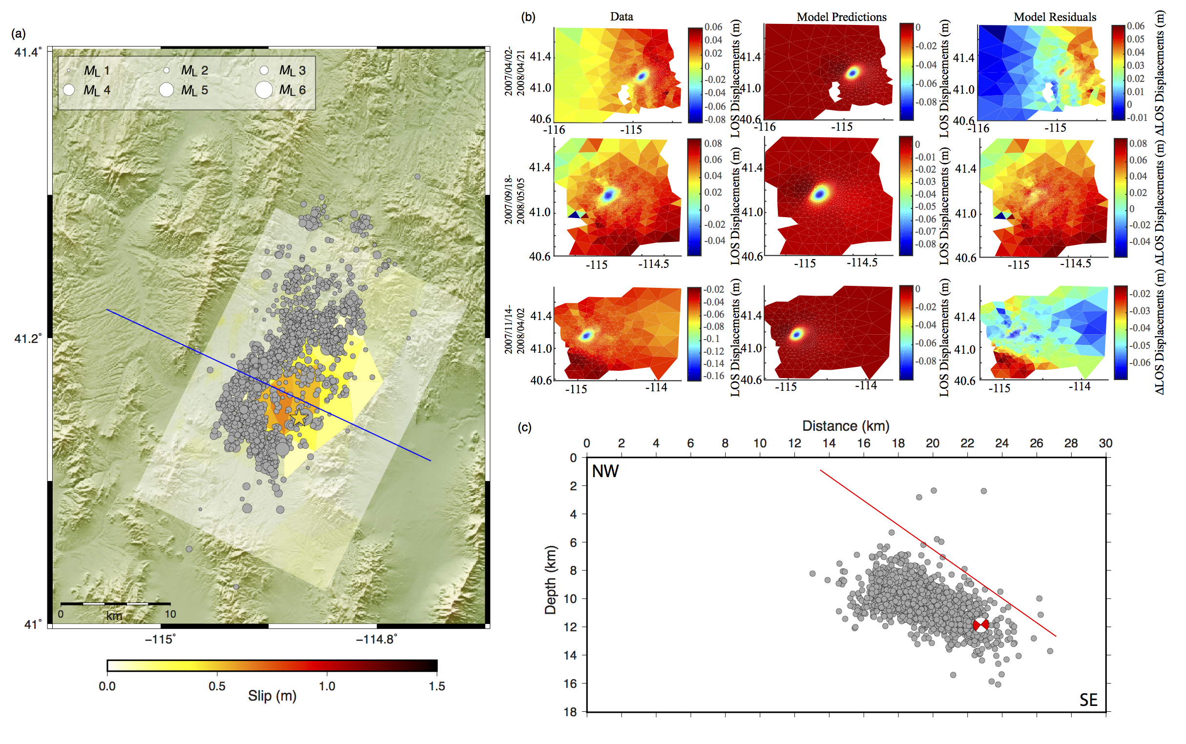
Figure S1. (a) Map view of the relocated aftershock locations with respect to slip distribution for inversion model 1. (b) Resampled interferograms, predicted displacements, and model residuals for the Interferometric Synthetic Aperture Radar (InSAR) model 1, described in Table 2 of the main article. Resampled interferograms denoted by their acquisition dates are detailed in Table 1 of the main article. Line-of-sight displacements are in meters, with negative displacements indicating line-of-sight increases (i.e., subsidence) and positive displacements indicating line-of-sight decreases (i.e., uplift). (c) Cross section along dip of the aftershock locations with respect to the slip distribution for the inversion model 1. The line shows the location of the fault plane.
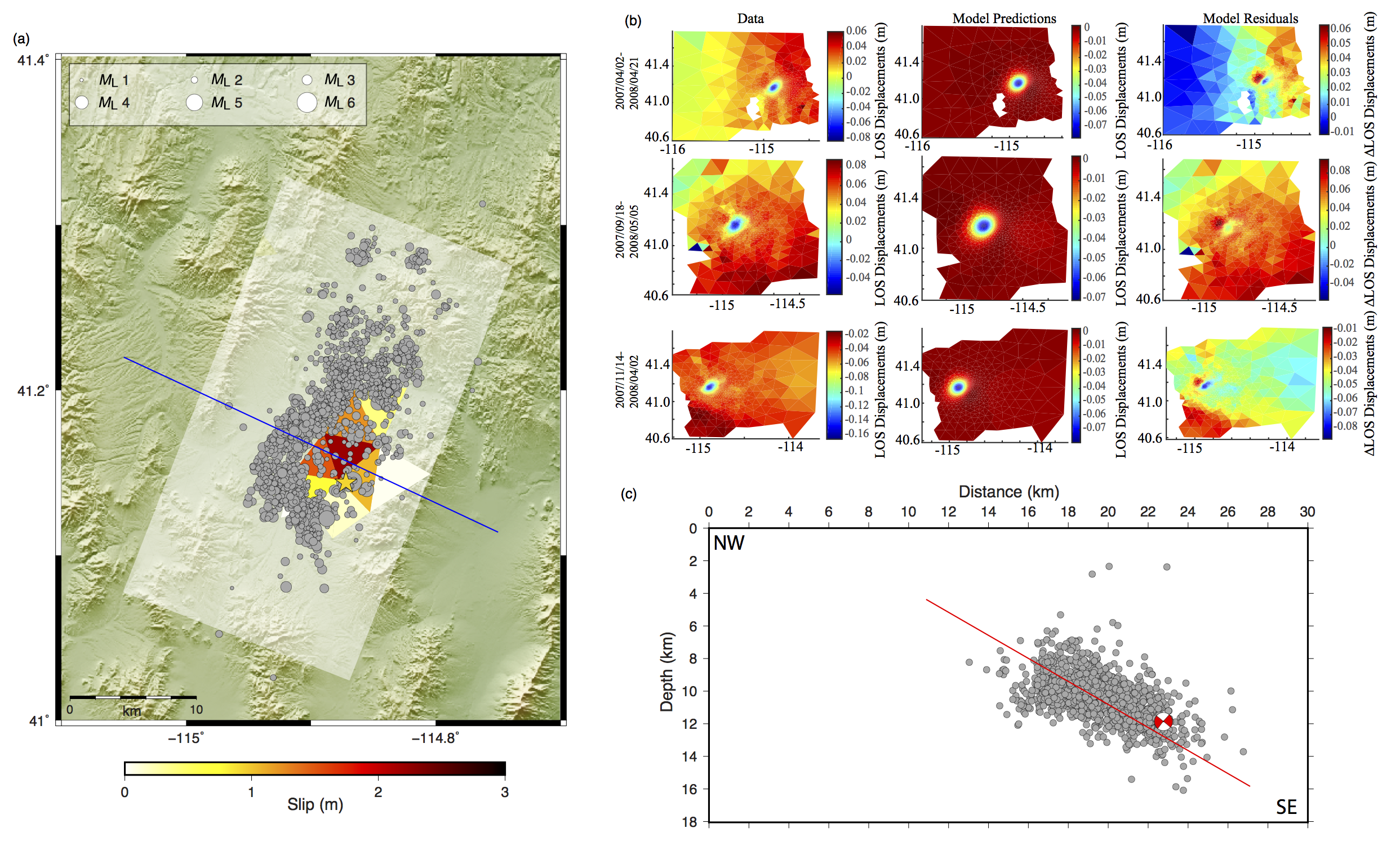
Figure S2. (a) Map view of the relocated aftershock locations with respect to slip distribution for inversion model 3. (b) Resampled interferograms, predicted displacements, and model residuals for the InSAR model 3, described in Table 2 of the main article. Resampled interferograms denoted by their acquisition dates are detailed in Table 1 of the main article. Line-of-sight displacements are in meters, with negative displacements indicating line-of-sight increases (i.e., subsidence) and positive displacements indicating line-of-sight decreases (i.e., uplift). (c) Cross section along dip of the aftershock locations with respect to the slip distribution for the inversion model 3. The line shows the location of the fault plane.
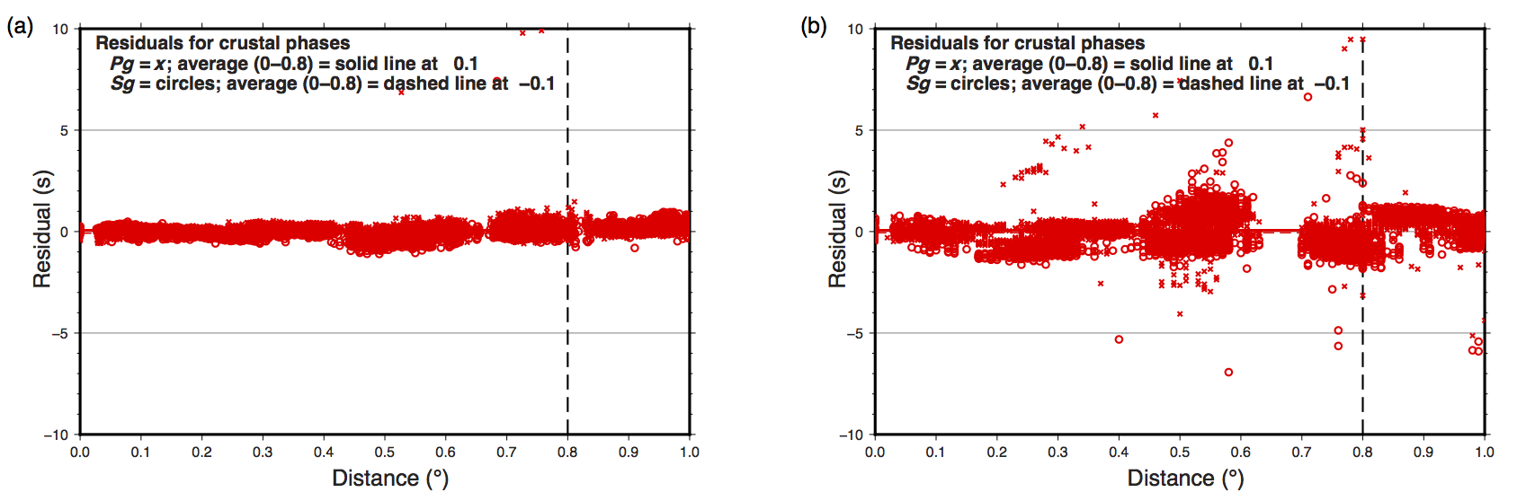
Figure S3. (a) Plot of residuals for near-source readings used in the HD relocation technique. Pg readings are represented by ×, and Sg readings are represented by circles. (b) Plot of residuals for near-source readings following an ~5 km shift of the HD relocations to the southeast. Pg readings are represented by ×, and Sg readings are represented by circles.
Figure S4. The transformations of the characteristic function used in the kurtosis detector for an event at 01:18:22 on 22 February at station M12A: (a) F1, kurtosis function; (b) F2, the kurtosis function cleaned of all strictly negative gradients; (c) F3, removal of linear trend; and (d) F4, amplitude scaling.
Baillard, C., W. C. Crawford, V. Ballu, C. Hibert, and A. Mangeney (2014). An automatic kurtosis‐based P‐ and S‐phase picker designed for local seismic networks, Bull. Seismol. Soc. Am. 104, no. 1, 394–409, doi: 10.1785/0120120347.
Fisher, R. A. (1921). On the “probable error” of a coefficient of correlation deduced from a small sample, Metron 1, 1–32.
Fouladi, R. T., S. K. Marani, and S. H. Steiger (2002). Moments of the Fisher transform: Applications using small samples, Proc. of AMSTAT Joint Statistical Meetings—Biometrics Section-to include ENAR & WNAR, 1032–1037.
Jordan, T. H., and K. A. Sverdrup (1981). Teleseismic location techniques and their application to earthquake clusters in the south-central Pacific, Bull. Seismol. Soc. Am. 71, no. 4, 1105–1130.
Lomax, R. G., and D. L. Hahs-Vaughn (2013). An Introduction to Statistical Concepts, Routledge, London.
[ Back ]