This electronic supplement contains forward modeling details, and model selection with Bayesian information criterion, and figures showing parameterization of the noise covariance matrix using autocorrelations of noise seismograms, the algorithm flowchart, and sampled centroid locations in four inversions of The Geysers earthquake.
Synthetic seismograms are computed as a linear combination of six elementary seismograms En, as defined in equation (2) in the main article. The elementary seismograms are computed as a convolution of the Green’s functions’ derivatives with the six elementary moment tensors (MTs) Mn:
(S1)
The elementary MTs are defined as
(S2)
and the seismic MT is their linear combination
(S3)
In our case, the model selection consists of determining the number of noise hyperparameters necessary to constrain the solution. The model selection process is necessary to determine the parsimonious (simplest) model that adequately explains the observed data (Maliverno, 2002). In Bayesian framework, the maximum-likelihood principle regularly leads to choosing the model with the highest dimension, but overparameterizing the model can lead to spurious features and unrealistically large uncertainties. We use an asymptotic point estimate of the Bayesian evidence called the BIC, which has been successfully employed in various geophysical studies (e.g., Dettmer et al., 2009; Pachhai et al., 2014).
The BIC is given by
(S4)
in which mml is the maximum-likelihood model vector, p(d|mml) its likelihood value, M is the number of model parameters, and N the number of data points. The first term in the equation reflects the fit to the data, and the second term includes a penalty for model complexity, including the number of data. Because the BIC is based on negative likelihood, the model with the lowest BIC is selected as the optimal model.
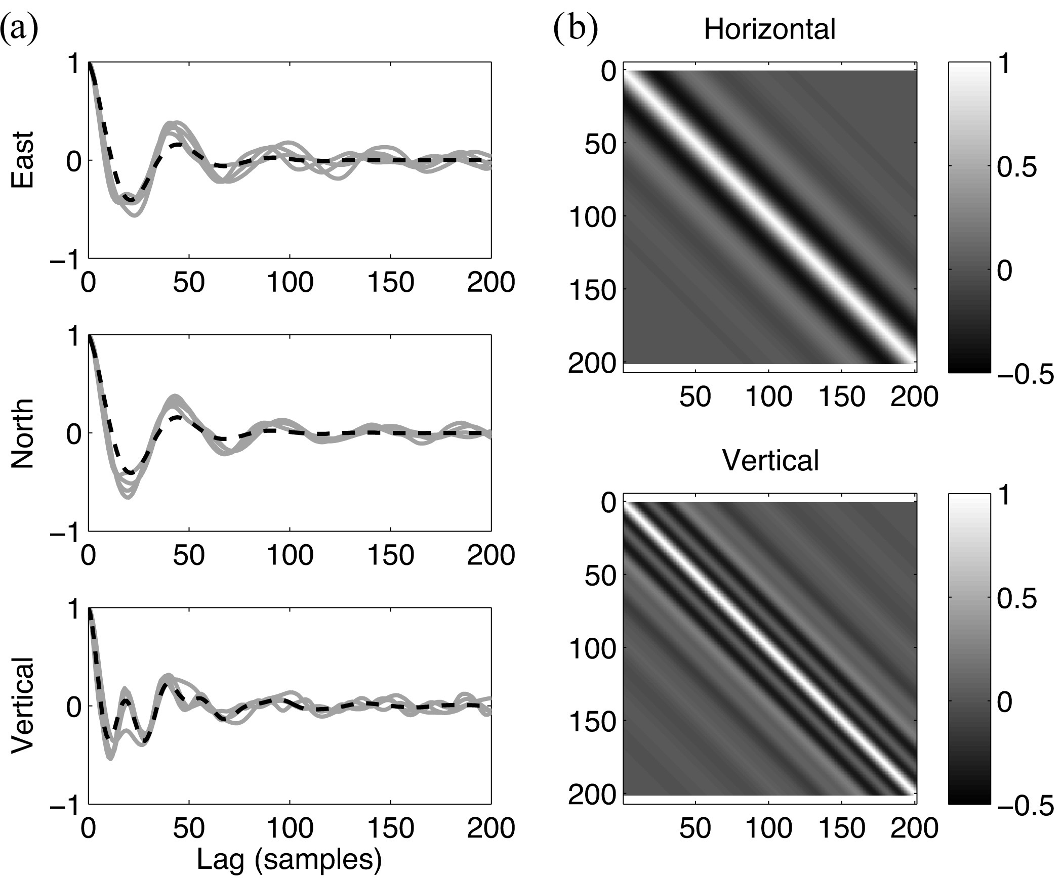
Figure S1. (a) (Gray) Autocorrelations of noise series on three seismogram components filtered between 20 and 50 s and (dashed black line) their fit using two attenuated cosine functions (cross-diagonal terms of the Cn matrices defined in equation 4 in the main article). (b) Covariance matrices Cn for the horizontal and vertical components.
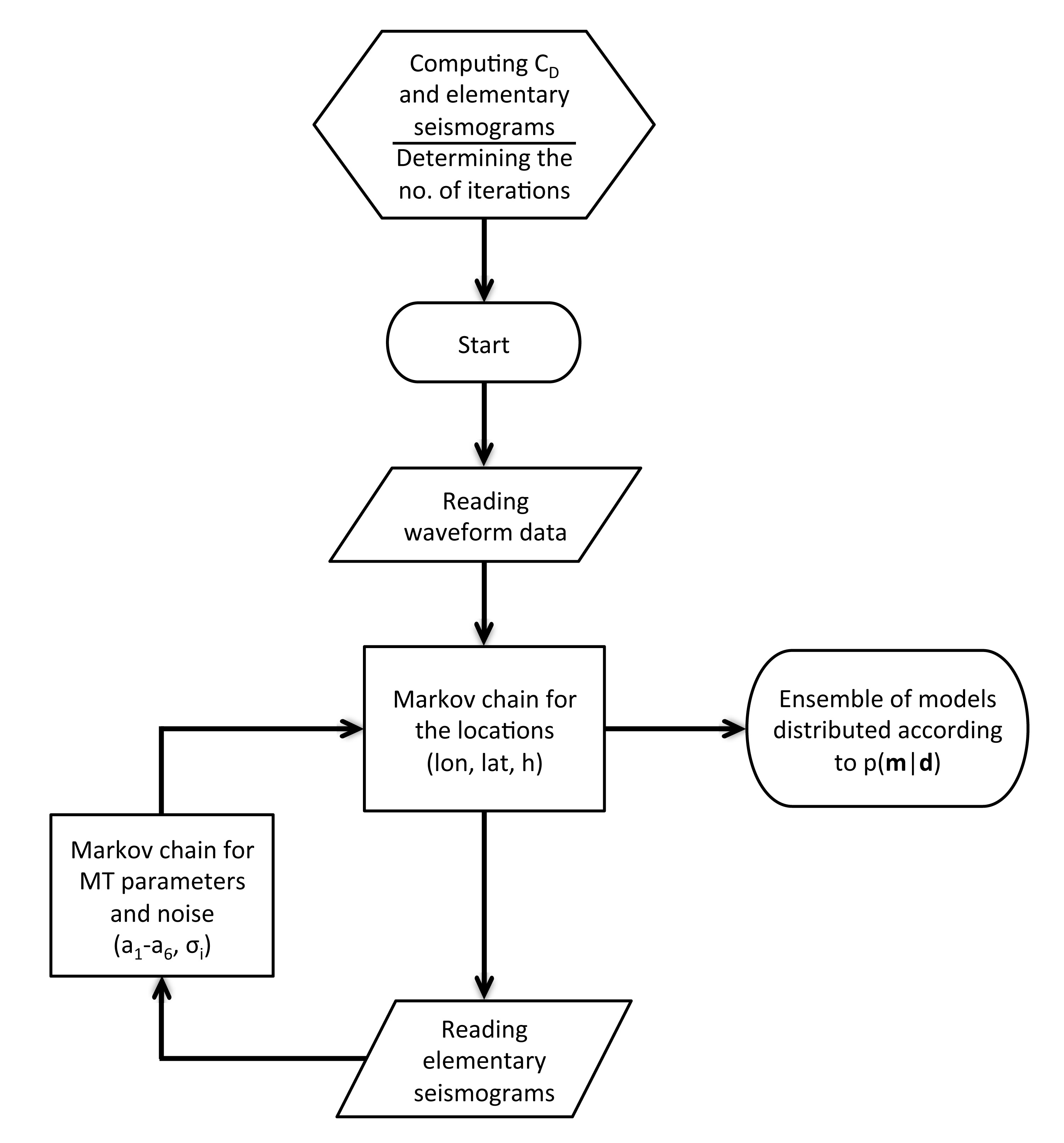
Figure S2. Flow diagram of the algorithm. The data covariance matrix and elementary seismograms are computed and the number of iterations determined prior to the inversion. Two Markov chains are used to sample the model space. For each location in the outer chain, six MT parameters (a1–a6) and the noise are sampled in a separate, inner chain. The number of noise parameters can be between one and the number of stations.
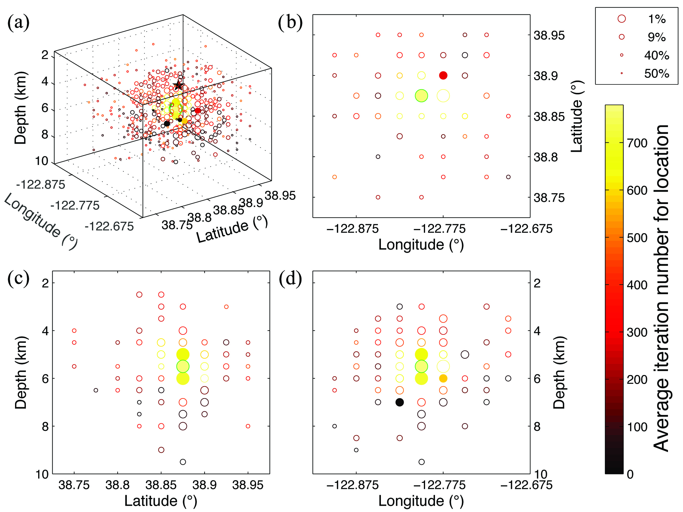
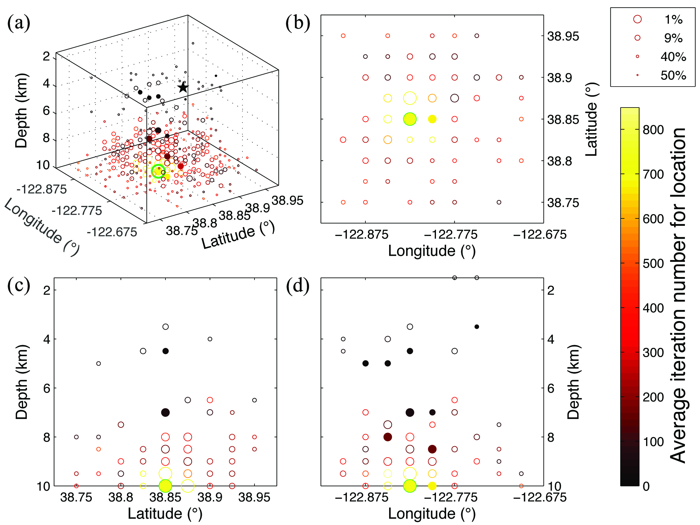
Figure S3. Centroid locations for 1000 iterations in the outer Markov chain for the inversion of The Geysers earthquake, assuming a diagonal covariance matrix and a common noise parameter. The average iteration number for each location determines its color. Open circles show all proposed locations, and full circles are the accepted ones. Symbol sizes are determined by the likelihood value (the 1% maximum a posteriori probability [MAP] locations are plotted with the largest circle, the next 9% with a smaller one, etc.). The black star is the Council of the National Seismic System (CNSS) hypocenter, and the green circle shows the MAP location. Locations are shown in (a) 3D and in (b)–(d) cross sections through the MAP source location.
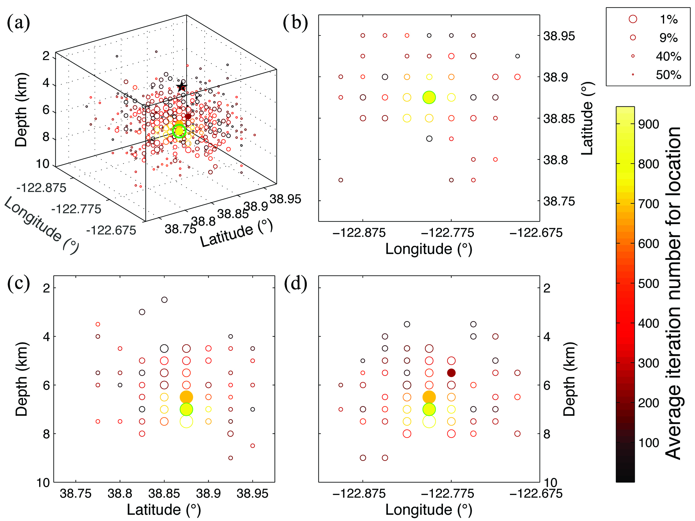
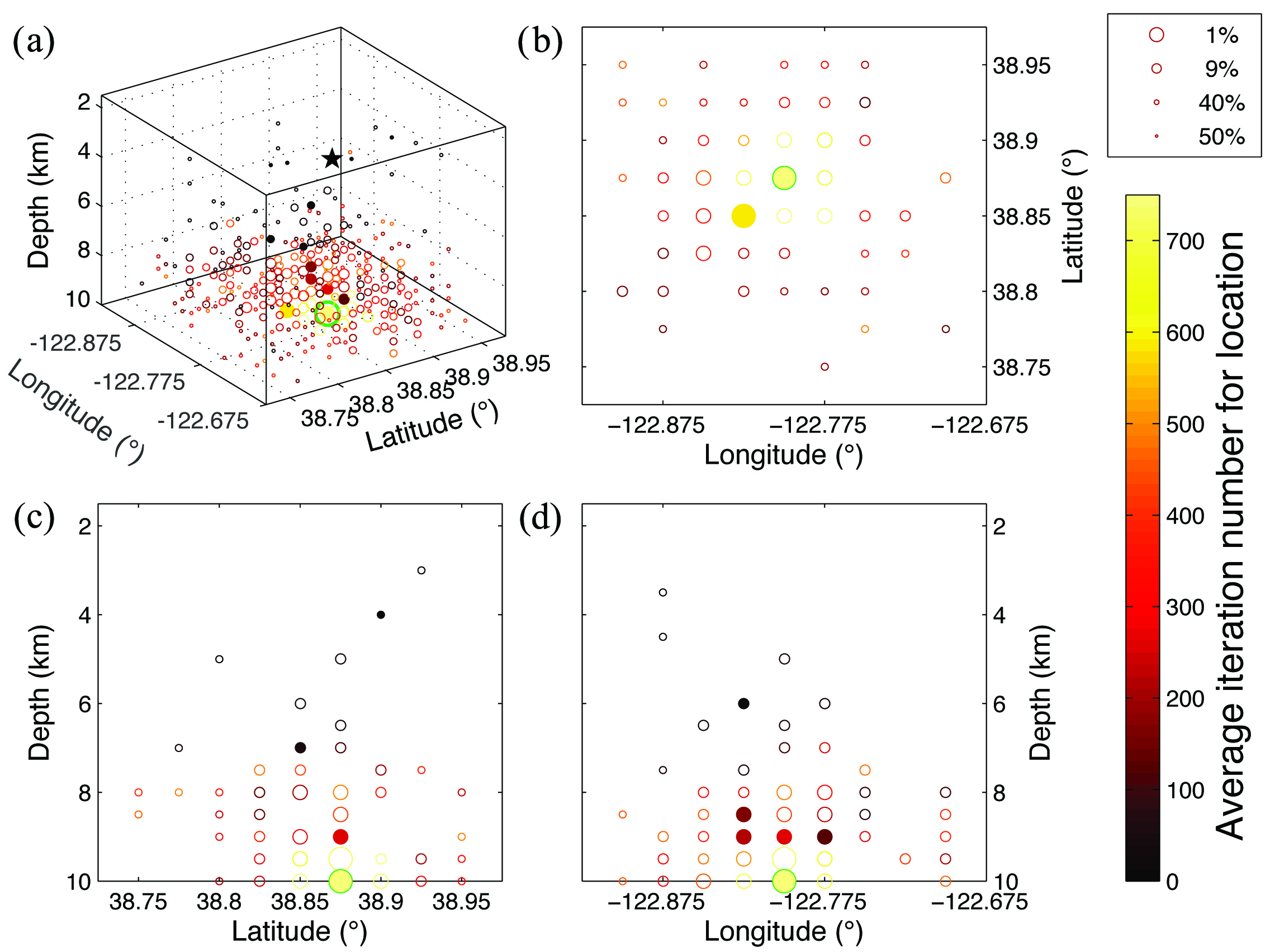
Figure S4. Sampled centroid locations for The Geysers earthquake in the inversion, assuming a diagonal covariance matrix and individual noise parameters (for details see the caption of Figure S3).
Figure S5. Sampled centroid locations for The Geysers earthquake in the inversion, assuming a covariance matrix with two attenuated cosine functions and a common noise parameter (for details see the caption of Figure S3).
Figure S6. Sampled centroid locations for The Geysers earthquake in the inversion, assuming a covariance matrix with two attenuated cosine functions and individual noise parameters (for details see the caption of Fig. S3).
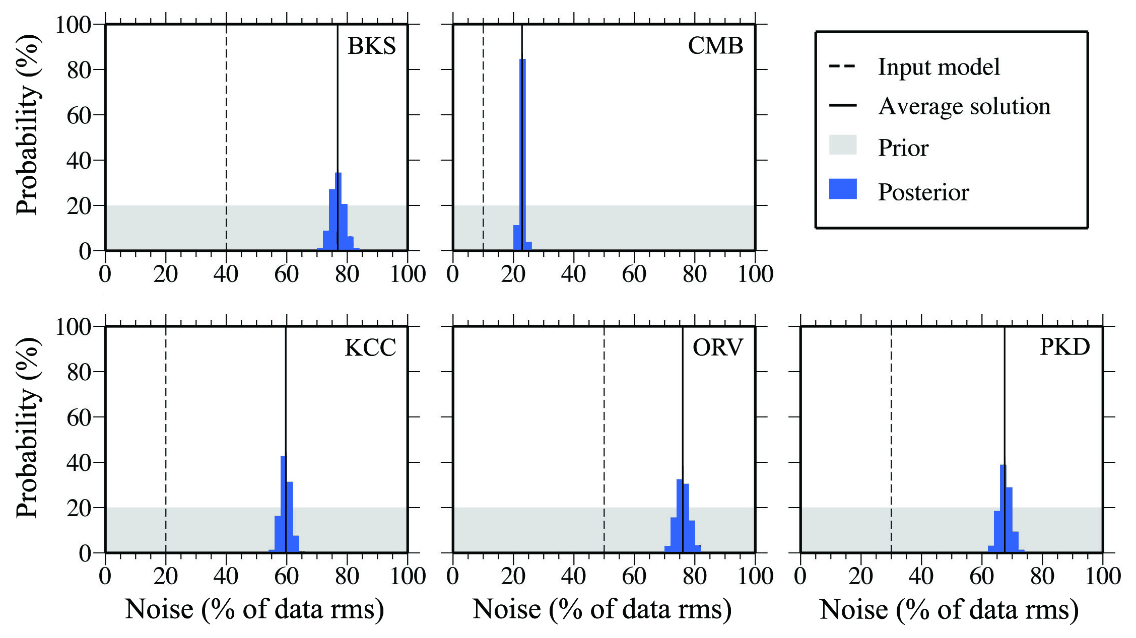
Figure S7. Posterior probability distributions of the noise hyperparameters, together with their input values (dashed lines) for the inversion with a diagonal covariance matrix in the synthetic test.
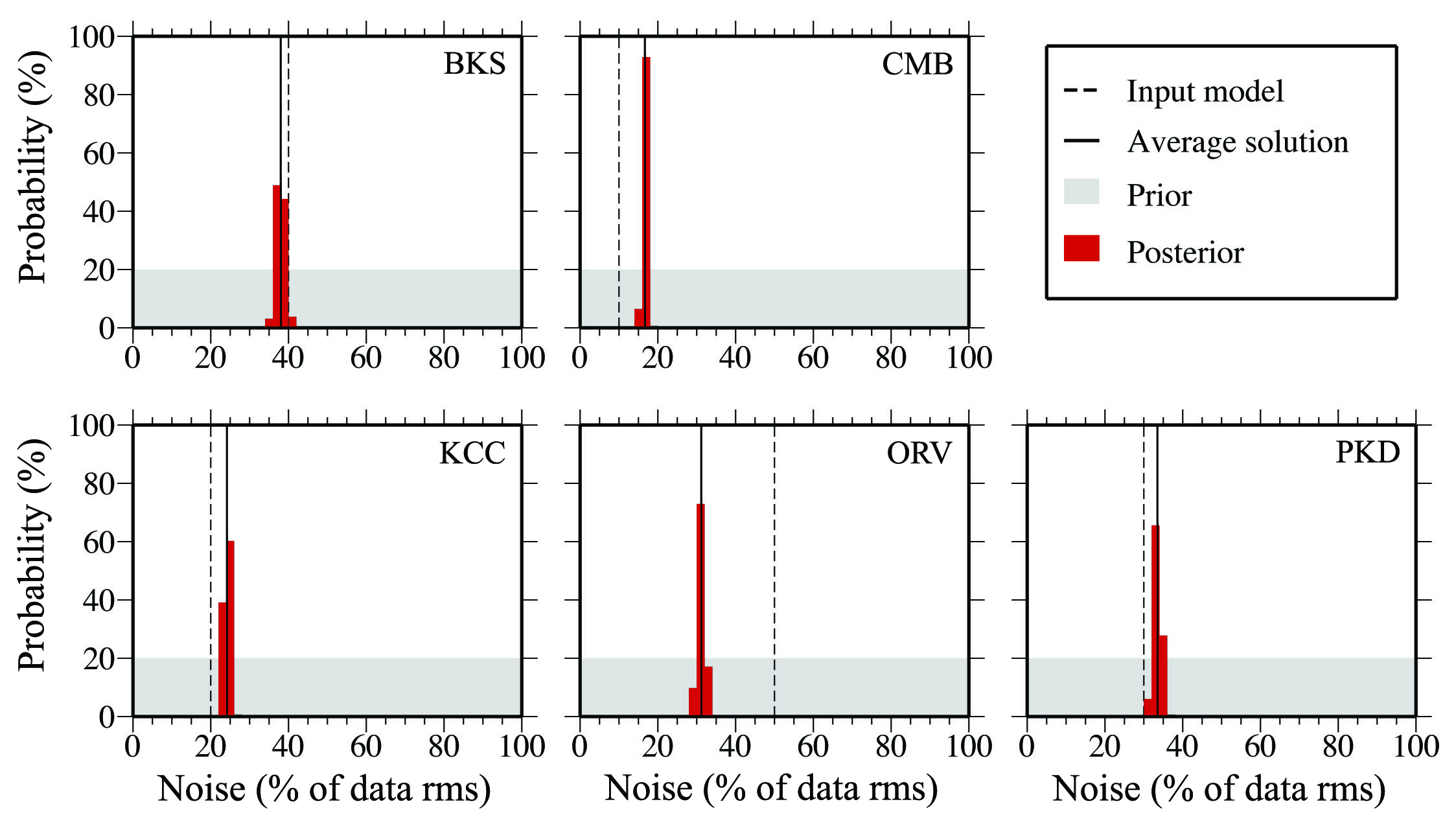
Figure S8. Posterior probability distributions of the noise hyperparameters, together with their input values (dashed lines) for the inversion with a cosine covariance matrix in the synthetic test.
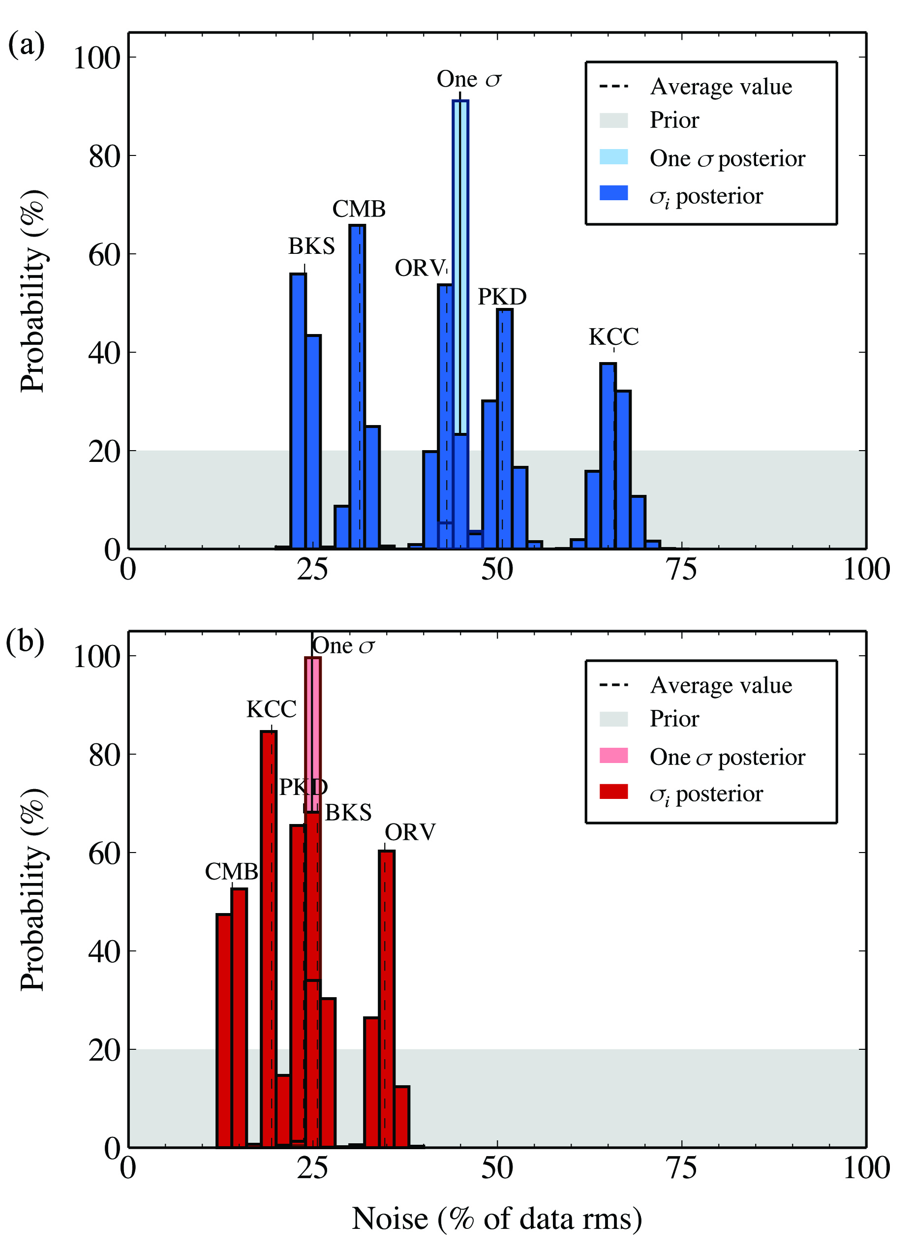
Figure S9. Posterior probability distributions of the noise hyperparameters in inversions with (a) a diagonal and (b) a cosine covariance matrix for the Long Valley caldera (LVC) earthquake.
Dettmer, J., S. Dosso, and C. Holland (2009). Model selection and Bayesian inference for high-resolution seabed reflection inversion, J. Acoust. Soc. Am. 125, no. 2, 706–716.
Maliverno, A. (2002). Parsimonious Bayesian Markov chain Monte Carlo inversion in a nonlinear geophysical problem, Geophys. J. Int. 151, no. 3, 675–688.
Pachhai, S., H. Tkalčić, and J. Dettmer (2014). Bayesian inference for ultralow velocity zones in the Earth’s lowermost mantle: Complex ULVZ beneath the east of the Philippines, J. Geophys. Res. 119, no. 11, 8346–8365.
[ Back ]