Electronic Supplement to
Development of a Time-Domain, Variable-Period Surface Wave Magnitude Procedure for Application at Regional and Teleseismic Distances, Part I: Theory

By David Russell

Digital Butterworth Filters

Introduction

This electronic supplement represents a second Appendix to my paper published in the Bulletin of the Seismological Society of America. The goal of this supplement is to highlight several important features of Butterworth bandpass filter design as it relates to surface wave analysis. Additionally, I provide an example Fortran program that can be used for Butterworth filtering of surface waves.

Software for constructing digital Butterworth filters is both widely available and simple to construct in terms of recursive infinite impulse response (IIR) filters. Kanasewich (1975) and many others discuss the construction of these filters in detail, and it is assumed that the reader is familiar with these algorithms. However, for constructing narrow band-pass filters, it is important to point out several issues in transforming continuous frequency domain filters into equivalent discrete digital time domain filters that can affect this study. To accomplish this, a review of the basic steps involved in Butterworth digital filter construction is appropriate.

Low-pass Filter Design

a. Start with the square of the transfer function for a low-pass filter (see equation 7 from paper):

₍₇₀₎

It is usually assumed that the square root of (70) represents the amplitude spectrum for a causal one-way Butterworth filter. However, for this study, only zero-phase non-causal filters are assumed, realized by applying a causal filter and then the conjugate reverse phase filter, so (70) represents the actual amplitude spectrum for the zero-phase filter.

b.Transform the filter into the Laplace domain with the variable substitution:

₍₇₁₎

c. Since (71) is a real function, it can be factored into a polynomial with its conjugate. The polynomial with roots on the left side of the complex plane can be used to construct a stable, causal digital filter:

₍₇₂₎

d. To transform H_L1 into a digital filter, use the bilinear z transform for a digital sampling interval dt

₍₇₃₎

e. Substitute (73) into (72) for an equivalent digital filter:

₍₇₄₎

Since z is just the Laplacian time shift operator, (74) can easily be set up as a recursive filter for an input signal X(z) as:

₍₇₅₎

f. To run the filter, transform (75) into the time domain, set initial conditions, and then update y(t) with past values as a recursive filter.

g. Finally, to run a zero-phase filter, reverse the filtered output y(t) into x(t), rerun (75), and then reverse the filtered output y(z) again. Again, notice that this will have a Butterworth filter amplitude spectrum given by (70).

For brevity, the above review is very condensed, and does not include methods to prewarp the Butterworth cutoff frequency w_c to account for non-linearity in the bilinear z transform, or methods to cascade the Laplace filter into smaller polynomials to provide more stable time domain filters. See Kanasewich (1975) for details.

Band-pass Filter Design

The standard approach to constructing a band-pass digital filter is similar to the steps for the low pass design, except for step b, where a Laplace transform is substituted which maps a normalized low-pass filter into a band-pass filter with corners w₁ and w₂.

a. The transform that maps the low-pass into band-pass is:

₍₇₆₎

b. Substituting (76) into (72) gives:

₍₇₇₎

c. Follow steps c through g under the low-pass design to realize the digital band-pass filter. Notice from (77) that when factoring the Laplace polynomials into conjugate functions in (72), there will be a factor of s²ⁿ in the numerator for the bandpass design. Again, see Kanasewich (1975) for detailed steps in constructing the digital filter.

Issues

One of the problems in using (77) in the construction of narrow-band time-domain recursive filters is the size of the Laplace polynomial. From (77) it can be seen that the maximum order of the polynomial in the denominator will be s⁴ⁿ instead of s²ⁿ as in the low-pass case. Although some stability can be gained be gained by cascading filters down to order 2, numerical instability can be a significant issue when using single precision processing with very narrow band-pass filters, when the filters are transformed into recursive form via (73) and (74). It is essential that computer routines that design and execute recursive band-pass filters with a basic form given by (77) be double precision for all floating-point operators. In addition, for long period calculations (>10 sec) it may be necessary to decimate the time series to 4 samples/sec or less to ensure stability.

Another issue in using (77) is the non-linearity in transforming a symmetric band-pass filter of the form given by (6) into the modified form (77). Recall that the original band-pass filter (6) was transformed into a low-pass filter by a simple shift in the frequency domain (equation 4). Equation (6) is:

₍₇₈₎

and can clearly be seen as symmetric about w₀. Now, it can easily be shown that (77) has the following form for its amplitude spectrum. Let w₁= w₀ - w_c, and w₂= w₀ + w_c. Then:

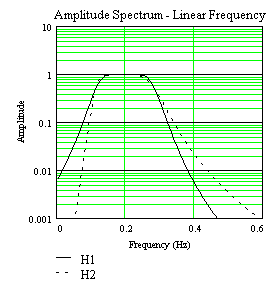
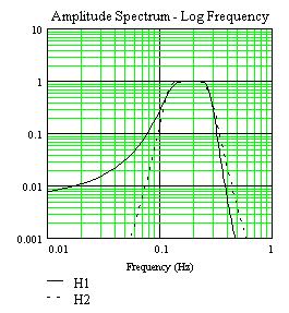
₍₇₉₎

For applications in this report, it is instructive to plot (78) and (79) in a worst case scenario, when the Butterworth cutoff frequency f_c has the maximum width and T is at the shortest period (5 seconds). Assume a 3^rd order Butterworth, and let f₀ = 0.2 Hz, f_c = 0.085 Hz. Plotting in linear and log frequency gives:

Figure ES-1.

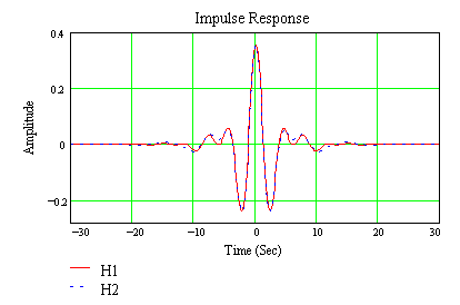
From Figure ES-1 it would appear that there is a significant effect due to how the band-pass filter is constructed; however, this is only pronounced due to expanding small changes with the logarithmic scale on the amplitude axis. Fast Fourier transforming the above frequency filters into the time domain to give the impulse response (Figure ES-2) shows that for purposes of measuring magnitudes, the above effects cause only 2^nd order changes in the time domain:

Figure ES-2.

Again, the above is the worst-case scenario. As the period increases and the filter width decreases, it can be shown that the difference between H₁ and H₂ decreases. In addition, synthetic seismograms with both source excitation and attenuation built in show less than 0.01 magnitude difference when filtered with H₁ and H₂.

Alternative Time Domain Recursive Filter

As an alternative to the standard IIR design given above, a different transformation can be used to design a recursive narrow-band filter which has the following advantages for operational processing:

- The filter response is equivalent to (78), following the exact theory in this report.

- The filter is built as cascaded first order filters instead of quadratic filters, thus improving the precision for very narrow-band applications.

- The filter returns a complex time-domain response, which can be used to extract the real filtered response and its envelope function without resorting to Fast Fourier transforms.

- The algorithm has been successfully tested for narrow-band applications in this report, for periods between 5 and 40 seconds, and sampling rates up to 40 samples/second, without requiring decimation.

NOTE: If large DC offsets are expected in the time series, it may be necessary to zero-mean the signal prior to filtering, since the amplitude of the filter is small but positive at 0 hertz.

The basic steps to construct the filter are:

a. Transform the low-pass into band-pass as:

₍₈₀₎

or equivalently:

₍₈₁₎

This formula represents a simple translation of a low-pass filter from the origin to w_0,resulting in a complex band-pass filter. Note that this is similar to using the positive half of the Fourier spectrum to form a complex time series, in order to calculate the Hilbert transform for the time series envelope function (Papoulis, 1962).

b. Substitute (80) into (70) for:

₍₈₂₎

c. Equation (82) can be factored into poles by first finding the poles p_j for the prototype low-pass filter in (82) (Kanasewich, page 181, 1975) and then substituting these poles into equivalent band-pass poles in (81) resulting in the form:

₍₈₃₎

d. Equation (83) can then be cascaded into simple causal first order filters:

₍₈₄₎

which can be transformed into time domain recursive filters of the form (75) using the bilinear z-transform (73).

e. Finally, after successively running the cascade recursive filters and then reversing for zero phase, the real part of the complex time series can be extracted for the narrow-band filtered signal, and the modulus of the series can be calculated for the envelope function.

Alternative Recursive Filter Coding Algorithm

To realize the above filter, a simple algorithm can be constructed which can be easily coded into C or FORTRAN code:

Define the following variables and vectors

INTEGER:

m = Butterworth order

n = number of time series points

j,k = counters

REAL

dt = sampling interval

ω₀ = Butterworth band-pass center frequency (2πf₀)

ω_c = Butterworth band-pass corner frequency (2πf_c)

xr(n) = input unfiltered time series

yr(n) = output filtered time series

er(n) = output envelope time series

ermx = maximum value of envelope series

COMPLEX DOUBLE PRECISION

p(m) = prototype low-pass Butterworth poles

s(m) = equivalent band-pass Butterworth poles

a1(m) = Z-transform recursive coefficients

a2(m) = Z-transform recursive coefficients

z1(n) = complex time series

z2(n) = complex time series

- Prewarp frequencies for bilinear z-transform:

- Calculate complex poles of Butterworth polynomial:

- Calculate complex bilinear z-transform recursive coefficients:

- Place input time series xr into real part of z1:

Calculate m cascaded first order filters:

j = 1,2,...m;

- Reverse complex time series:

- Calculate m reversed first order filters (a1^*,a2^* complex conjugates of a1,a2):

j = 1,2...m;

- Reverse complex time series:

- Calculate output realtime series, envelope, and envelope maximum:

---

An example Butterworth filtering program written in Fortran can be found here [Fortran source code text file; 8 K].

 

---

[ Back ]