
May/June 2001
Steve Malone
E-mail: steve@geophys.washington.edu
Geophysics, Box 351650
University of Washington
Seattle, WA 98195
Phone: (206) 685-3811
Fax: (206) 543-0489
FOREWORD
The Electronic Seismologist (ES) has been known to actually do some research in the field of seismology from time to time. As an operator of a seismic monitoring network the research done often is related to the seismicity of the monitored region. Detecting changes or trends in seismicity is relevant to earthquake and volcano hazards, but are the trends detected real or only an artifact of changes in the network operating parameters? Because all seismic networks evolve, change staff, change software and hardware, there is always the nagging feeling, if not outright knowledge, that interesting patterns in the catalog reflect network changes rather than changes in the Earth. How can one tell the difference?
The ES is happy to report that there is a handy-dandy software package ideally suited to answering exactly this question (and many others). ZMAP, developed by Stefan Wiemer, allows the user to examine an earthquake catalog from many different angles. Not only does it include the traditional map, cross-section, and time sequence parameters, but also several others, such as event size and mechanism. These can be combined in interesting ways to present the user with different "views" into the data. Considerable seismological acumen lies behind the use and presentation of these parameters, which helps the user get the most out of the analyzed catalog. ZMAP is fairly intuitive to use and produces attractive output. In fact, the ES actually has fun "playing" with it and gets useful results besides. Perhaps one of the best ways to get a sense of how ZMAP might be used is to take a tour of case studies. The following includes many examples, and if they're not enough there are a slew of references where one can find more. In his traditional groveling way the ES has prevailed on Stefan Wiemer to write this month's column for him.
A SOFTWARE PACKAGE TO ANALYZE SEISMICITY: ZMAP
Stefan Wiemer
Institute of Geophysics
ETH Hoenggerberg
CH-8093, Zurich
Switzerland
Telephone +41 633 3857
stefan@seismo.ifg.ethz.ch
Introduction
Earthquake catalogs are probably the most fundamental products of seismology and remain arguably the most useful for tectonic studies. Modern seismograph networks can locate up to 100,000 earthquakes annually, providing a continuous and sometime overwhelming stream of data. ZMAP is a set of tools driven by a graphical user interface (GUI), designed to help seismologists analyze catalog data. ZMAP is primarily a research tool suited to the evaluation of catalog quality and to addressing specific hypotheses; however, it can also be useful in routine network operations. Roughly 100 scientists worldwide have used the software at least occasionally. About 30 peer-reviewed publications have made use of ZMAP. A comprehensive listing of ZMAP features is given in Table 1.
| Table 1 | ||
| Comprehensive Listing of ZMAP Functions and Relevant References | ||
| Tool | Objective | Comments and References |
| Histograms | Histograms of magnitude, depth, time, hour of the day | |
| Data Import | Data import as ASCII, column-separated files, using one of several existing input format filters or a custom-designed one. | |
| Catalog Comparison | Identification of identical events in two catalogs spanning the same region. Plot of the mean difference in magnitude, depth, location, and temporal evolution of these differences. Map of hypocenter shifts. | |
| Time Series Analysis | Cumulative number of events, time-depth plots, time-magnitude plots, cumulative moment release. Significance of rate changes using z, ß, and translation into probability. | |
| Data Subset Selection | Select data inside or outside polygons, cut in magnitude, depths, or time. | |
| Maps | Maps of seismicity; legend by time, depth, or magnitude. 3D view and rotation hypocenters. Cross-sections with one or multiple segments. Link to M_Map toolbox. Import and plot topography files (ETOPO5, ETOP2, GTOPO30, USGS 1deg). Import hierarchical coastline data. | |
| GENAS | Evaluate homogeneity of magnitude reporting with time. Compute magnitude signatures; compare FMS for two periods and model rate changes. | (Habermann, 1983, 1986, 1987; Zuñiga and Wiemer, 1999; Zuñiga and Wyss, 1995) |
| Declustering | Separation of dependent and independent seismicity, identification of clusters. Based on Reasenberg's algorithm. | (Reasenberg, 1985) |
| Mapping Seismicity Rates | Map seismicity rates in map view, cross-section, or 3D. Animate maps of z and ß values as a function of time. Compute alarm cubes, explore 6D parameter space. | (Maeda and Wiemer, 1999; Wiemer and Wyss, 1994; Wyss et al., 1996; Wyss et al., 1997a; Wyss and Wiemer, 1997, 2000; Wyss and Martyrosian, 1998) |
| Aftershock Decay Rates | Estimate aftershock decay rates based on modified Omori law. Compute probabilistic aftershock hazard. Compute maps and cross-section of p values and aftershock probabilities. Link to ASPAR software. | (Kisslinger and Jones, 1991; Reasenberg and Jones, 1989, 1990; Wiemer, 2000; Wiemer et al., 2001) |
| Frequency-magnitude Distribution | Estimate a and b values and uncertainties using maximum likelihood or weighted least squares as a function of depth, time, and magnitude. Map b and a values in map view, cross-section, or 3D. Compute local recurrence time maps. Differential b value maps for two periods. Create synthetic catalog with constant b. | (Wiemer and Benoit, 1996; Wiemer and McNutt, 1997; Wiemer and Wyss, 1997; Wyss et al., 1997b) |
| Magnitude of Completeness | Estimate magnitude of completeness based on the deviation of the FMD from a power law. Analyze Mc as a function of time or depth. Map Mc in map view or cross-section. | (Wiemer and Wyss, 2000) |
| Fractal Dimension | Compute the fractal dimension of hypocenters based on the correlation integral. Create maps and cross-sections of the fractal dimension. | (Sammis et al., 2001) |
| Quarry Maps | Compute and map out the daytime to nighttime ratio of events in order to identify explosion. Dequarry catalogs by removing daytime events at significantly anomalous nodes. | (Wiemer and Baer, 2000) |
| Time to Failure | Estimate the time to failure based on accelerated moment release or Benioff strain. | (Bufe et al., 1994; Bufe and Varnes, 1996; Jaume and Sykes, 1999; Varnes, 1989) |
| Stress Tensor | Inversion for the best fitting stress tensor using Michael's or Gephart's approach. Uncertainty estimation. Maps/cross-sections of stress orientation and variance/heterogeneity of the stress field. Maps of the temporal change in the stress field. | External call, requires compilation of FORTRAN and C code. (Gephart, 1990a; Michael, 1984; Wiemer et al., 2001) |
| Cumulative Misfit | Compute the cumulative misfit to a predefined stress tensor. Cumulative misfit as a function of time, depth, magnitude, lat, lon, or in map view or cross-section. | External call, requires compilation of FORTRAN and C code. (Lu et al., 1997; Wyss and Lu, 1995) |
ZMAP was first published in 1994 and has continued to grow over the past seven years. Concurrent with this article, we are releasing ZMAP v. 6, which contains numerous bug fixes and a few new features, as well an updated manual.
This paper illustrates some of the capabilities and applications of ZMAP by summarizing a few case studies that have been published previously. The examples include (1) catalog quality assessment and data exploration; (2) mapping b values beneath a volcano to infer information about the location of magma; (3) estimating seismicity rate changes caused by a large earthquake; (4) stress-tensor inversion on a grid to measure the heterogeneity of a stress field; and (5) mapping the magnitude of complete reporting.
The Philosophy of ZMAP
Matlab-based, open-source code. ZMAP is written in Mathworks' (http://www.mathworks.com) commercial software language, Matlab®, a package widely used among researchers in the natural sciences. Users must purchase a Matlab license to run ZMAP. Although ZMAP is written in Matlab, no knowledge of the Matlab language is needed since ZMAP is GUI-driven. The ZMAP code is, however, open, and users are welcome to modify or supplement as desired by diving into the guts of the numerous scripts (about 80,000 lines of native code in 600 scripts). ZMAP should run on all platforms supported by Matlab. We have tested it under Unix, Linux, PC, DEC ALPHA, and Macintosh computers (Caveat: Some code, such as stress-tensor inversions, requires the compilation of external FORTRAN or C programs).
Interactive data exploration. ZMAP combines many standard and advanced seismological analysis tools, aspiring to make data exploration easier and more efficient. The user can quickly select subsets in space, time, and magnitude, plot histograms, compute b or p values, compare the frequency-magnitude distributions of different time periods and locations, compare daytime versus nighttime activity, compute the fractal dimension of hypocenters, create cross-sections, overlay topography, compute stress-tensor inversions, and much more (Table 1). The ability to apply and combine these analysis tools within one software platform helps users explore or mine their data in detail. A typical snapshot of some ZMAP windows is shown in Figure 1.
|
|
Mapping seismicity parameters. Identifying and evaluating spatial and temporal variations in seismicity is one of the primary research objectives of ZMAP. By creating dense spatial grids and sampling overlapping volumes of circular (2D) or spherical shape (3D), users can map such parameters as seismicity rate changes, b values, p values, stress-tensor orientations, and the magnitude of completeness. In any map, the user can interactively view the source of the parameter under investigation (e.g., a frequency-magnitude plot) and compare neighboring volumes.
Maps are computed on an interactively defined grid that generally excludes low-seismicity areas (Figure 2B). There are two methods programmed into ZMAP to map seismicity: using either constant radii or a constant number of samples. The first method produces maps with a continuous spatial resolution but varying sample sizes. Consequently, uncertainties can vary significantly in space. A constant sample size, on the other hand, results in more homogeneous uncertainties, but the resolution, which is inversely proportional to the density of earthquakes, will vary across the region of interest. This is demonstrated in Figure 2B, where we plot a cross-sectional view of the hypocenters beneath Mt. St. Helens. Circles plotted at selected nodes indicate the volumes sampled around each particular node. The grid spacing is generally chosen such that the volumes overlap significantly, providing a natural smoothing of the results.
|
|
Sample Applications
The sample applications shown below are intended to illustrate some of the capabilities of ZMAP. The images shown were all created with ZMAP, edited manually using the Matlab edit capabilities, and then imported as JPEG files or Windows metafiles into PowerPoint to be arranged on a page. The online help (http://seismo.ethz.ch/staff/stefan/) discusses how each analysis was performed. Most case studies are taken from published work that discusses the science and interpretation in detail.
Assessing Catalog Homogeneity and Interactive Data Exploration
ZMAP can be used to investigate or monitor the reporting history and health of a seismic network. The user can address questions such as: Did the detection threshold change in a particular area at a certain time? Did the meaning of magnitude change? A long list of man-made changes in earthquake catalogs has by now been documented (Habermann, 1983, 1986, 1987, 1991; Wyss and Toya, 2000; Zuñiga and Wiemer, 1999; Zuñiga and Wyss, 1995). These changes in the reporting rate can be introduced by modifications to the network and can either mask or mimic natural changes in the seismicity. Using GENAS (investigation of rate changes as a function of magnitude threshold), magnitude signatures, b-value curves, and maps of rate changes one can attempt to unravel the reporting history of earthquake catalogs as a function of space and time.
A simple example of network quality assessment is shown in Figure 1. The cumulative number of events along the creeping section of the San Andreas Fault north of Parkfield (0 < M < 1.2) indicates a decrease in the rate of small earthquakes around 1995. The cumulative and noncumulative number of events as a function of magnitude is compared for two periods (1990-1995 and 1995-2000). This plot reveals that the number of events with M < 1.2 dropped by about 65% in the latter period, whereas no change is observed for larger earthquakes. The simplest explanation of this pattern is that there was a change in the network configuration or processing strategy which decreased the detection ability of the CALNET network in the creeping section after 1995.
The b Value beneath Mount St. Helens
ZMAP is frequently used to facilitate spatial mapping of the b value in various seismotectonic regimes. The b value, defined as log10N = a - bM, where N is the cumulative number of earthquakes, and a and b are constants related to the activity and earthquake size distribution, respectively (Gutenberg and Richter, 1944; Ishimoto and Iida, 1939), has been shown to vary spatially on scales of hundreds of meters to tens of kilometers (e.g., Wiemer and Benoit, 1996; Wiemer and Katsumata, 1999; Wiemer and McNutt, 1997; Wiemer et al., 1998; Wiemer and Wyss, 1997; Wyss et al., 2000). These variations are related to differences in stress, pore pressure, and material heterogeneity and therefore can give important constraints when analyzing the seismotectonics and hazard potential of a region. High b values are often correlated with the presence of magma in volcanic regions (Jolly and McNutt, 1999; Murru et al., 1999; Power et al., 1995; Wiemer and McNutt, 1997; Wiemer et al., 1998; Wyss et al., 1997b). We present as an example data from Mount St. Helens (Wiemer and McNutt, 1997), using earthquakes of magnitude 0.4 and greater recorded by the local network during the period of 1988-1995, a total of about 2,000 events.
Using ZMAP, we can investigate spatial variations in b value in one, two, and three dimensions. Looking at b values as a function of depth (Figure 2A), we find high values of b (b > 1.1) at around 2.5 km and deeper than 6 km below sea level. For this analysis, a constant number of events per sample (100) is used, incremented downward by 25 events for each step. The two-dimensional gridding along a 2-km-wide, north-south-trending cross-section (Figure 2B) shows that indeed the b value exhibits its strongest variations as a function of depth. The orientations of the cross-section and the hypocenters are shown in Plate 1A. Finally, a three-dimensional gridding is applied and a perspective view of the topography of Mt. St. Helens added (Plate 1A).
|
|
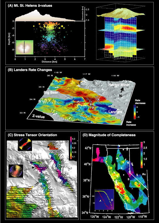
For this particular case study, the 3D view contributes little to the scientific analysis of the data, since the seismicity distribution is largely one-dimensional. Creating an artistic image such as Plate 1A often requires some effort using the editing options in Matlab in order to get the perspective and the light properties right; however, the outcome may be worth the effort. To verify that the mapped differences in b value are indeed significant, we plot in Figure 3 comparisons of b values for the shallowest earthquakes (b = 0.77) and the depth range 2-3 km (b = 1.82). The difference in the frequency-magnitude distributions is clear to the eye and highly statistically significant, which is established using a statistical test proposed by Utsu (1992).
|
|
The scientific interpretation of these results, of course, still depends on the ingenuity of the analyst. Based on the analysis of the b value at Mt. St. Helens and nine other volcanoes (Jolly and McNutt, 1999; Murru et al., 1999; Power et al., 1998; Wiemer and McNutt, 1997; Wiemer et al., 1998; Wyss et al., 1997b; Wyss et al., 2000), we have proposed that (1) the b value underneath volcanoes is not generally higher, but pockets of high b exist in otherwise quite normal crust. (2) These pockets of high b may signal the presence of magma, since in the vicinity of a substantial body of magma, high pore pressure and high temperature gradients favor high b values. The absence of high b values, on the other hand, should be taken as a strong indication that no substantial magma body is present near this volume.
Mapping Seismicity Rate Changes
Measuring changes in the seismicity rate is a tricky business. It is important, because rate changes are believed to be directly related to changes in stress or pore pressure (Dieterich, 1994; Dieterich and Okubo, 1996). Applications include constraining stress changes caused by Coulomb failure (Harris, 1998; Stein et al., 1992) or precursory rate changes (Katsumata and Kasahara, 1996; Maeda and Wiemer, 1999; Wiemer and Wyss, 1994; Wyss and Habermann, 1988; Wyss and Martyrosian, 1998; Wyss and Wiemer, 1997). Measuring rate changes is difficult because (1) artificially introduced rate changes are common in seismicity rates, (2) aftershocks and other clustered events should be excluded before measuring background rates, and (3) defining the significance of an observed rate change is not simple.
ZMAP helps in various ways to deal with each of these obstacles. As an example, we investigate the change in the seismicity rates in southern California associated with the 1992 M 7.3 Landers earthquake. For details, please refer to Wyss and Wiemer (2000). The first task is preparing a homogeneous input data set. We spatially map the magnitude of complete reporting, Mc, for different periods. Areas with higher Mc, such as the offshore region and south of the Mexican border, can thus be excluded based on an objective criterion. We next test for the presence of explosions in the study region by spatially mapping the daytime to nighttime ratio of events. A significantly enhanced ratio is indicative of quarry blast contamination that often remains in the data regardless of the network operator's efforts (Wiemer and Baer, 2000). We identify a number of explosion-prone regions, which we exclude. By studying the homogeneity of reporting as a function of time and magnitude, we search for artificial rate changes in the data and the suitable overall Mc cut-off. Finally we settle for a data set for the period 1985-1999.8 (before the Hector Mine earthquake) with an overall Mc of 1.7. This data set is then declustered using Reasenberg's (1985) approach.
We spatially map the remaining seismicity rate changes, comparing the periods 1985-1992.48 and 1992.6-1999.8, using constant sample volumes of 20 km radius and a grid spacing of 5 km. Two different statistical functions have been implemented in ZMAP to measure the significance of rate change: z values (Habermann, 1981, 1988) and ß values (Matthews and Reasenberg, 1988; Reasenberg and Simpson, 1992). A map of rate changes measured by z is shown in Plate 1B. Red colors signify rate increases, blue colors rate decreases. The map is wrapped on top of the GTOPO30 topography; this is possible in ZMAP only when the Matlab mapping toolbox is available. We can interactively select circular or polygonal volumes from the map and view the cumulative number of events as a function of time and the z values that measure rate changes (Figure 4).
|
|
The pattern of rate change mapped by this technique is quite remarkable, since it reveals long-range (> 100 km) and long-duration (> 7 years) rate changes associated with the 1992 Landers main shock. The pattern of increased and decreased seismicity matches qualitatively the predicted rate changes caused by the combined static and dynamic stress changes predicted for the Landers rupture (Stein et al., 1992). In order to establish a significant rate decrease, it is generally necessary to compare observations for several years.
Stress Tensor Inversions
In addition to hypocenter information, ZMAP can be used to analyze focal mechanism data either by analyzing the cumulative misfit of a set of focal mechanisms to a given stress tensor (Lu and Wyss, 1996; Lu et al., 1997; Wyss and Lu, 1995), or by computing inversions for the best-fitting stress tensor. Two inversion programs are called from ZMAP, Michael's (Michael, 1984, 1987a, 1987b, 1991; Michael et al.) and Gephart's (Gephart and Forsyth, 1984; Gephart, 1990a; Gephart, 1990b). ZMAP allows the computation of individual stress-tensor inversions, stress tensor as a function of time and depth, and inversions on a grid in either map view of cross-section (using Michael's method only).
An example application, again for southern California, is shown in Plate 1C. We use the relocated set of focal mechanisms from 1992.48-2000.5 by Hauksson (2000), with a solution misfit < 0.1. First we create a grid with a 2 X 2 km spacing, excluding areas of low seismicity. The nearest 100 earthquakes to each node are sampled and their focal mechanisms inverted using Michael's approach. The resulting directions of the principal stress axes, ![]() 1, are plotted as lines on a map underlain by topography. We further color-code the variance of the resulting inversion at each node. Blue to purple colors indicate a high variance (i.e., heterogeneous stress field). The two inserts show the individual inversion results and their uncertainties, obtained using a bootstrapping approach (Michael, 1987a).
1, are plotted as lines on a map underlain by topography. We further color-code the variance of the resulting inversion at each node. Blue to purple colors indicate a high variance (i.e., heterogeneous stress field). The two inserts show the individual inversion results and their uncertainties, obtained using a bootstrapping approach (Michael, 1987a).
The overall stress directions obtained agree reasonably well with a more detailed study by Hauksson (1994). Results suggest that areas that experience a high slip during the main shock show a more heterogeneous stress field which cannot be fit by a single stress tensor, whereas areas outside the main rupture show a low variance, hence a more homogeneous stress field (Wiemer et al., 2001).
Mapping Minimum Magnitude of Completeness (Mc)
The quality of all regional and local earthquake catalogs decreases with distance from the center of the network. Obvious boundaries of deterioration are coastlines, international borders, and seams between networks. To avoid problems that could be introduced in seismicity studies by heterogeneity of Mc, ZMAP allows the user to map Mc to define the spatial extent of the high-quality part of the catalog (e.g., Wiemer and Wyss, 2000). The technique used most frequently to assess Mc is based on estimating it from the FMD itself. This is often done in seismicity studies by visual examination of the cumulative or noncumulative FMD; however, we prefer to apply a quantitative criterion, where we measure the goodness of fit to an assumed power law (Wiemer and Wyss, 2000). An example of a map of Mc for the western U.S., based on the CNSS catalog for the period 1995-2000, is shown in Plate 1D. Mc ranges from > 2.5 offshore Mendocino to < 1 in central California.
Obtaining ZMAP, Documentation, and Support
ZMAP is freely available on the Internet. Please refer to http://seismo.ethz.ch/staff/stefan to download the current version of ZMAP (version 6). The compressed files are about 5 Mb and should run under Matlab 5.x and 6.0. Other resources on the ZMAP home page include a list of papers published using ZMAP, a collection of sample data files, and a collection of presentations made using the ZMAP software. If your Internet connection does not allow downloading via the Internet, we can send you a CD-ROM version of ZMAP. Please contact stefan@seismo.ifg.ethz.ch.
The only support currently available beyond the online documentation is contacting me via e-mail. Help requests will be addressed as quickly as possible, but as they increase in volume this may become unmanageable. A ZMAP help e-mail list is being considered.
Known Problems
From the responses from the 100+ scientists using ZMAP, it is clear that, although designed to work on any Matlab-supported platform, some users experience problems while running various functions. Others become frustrated with the variable robustness of certain features of ZMAP and the occurrence of errors. Although the source code is open, it is not trivial to find the appropriate script and variable in order to extend or improve ZMAP.
As with any software, the garbage in-garbage out principle applies to ZMAP. If you try, for example, to estimate spatial and temporal variations of b values and your catalog contains only 200 events, you may get colorful maps but their meaning is questionable at best.
The Future of ZMAP
The future of ZMAP is somewhat unclear. There will likely be occasional future updates of ZMAP, largely driven by research interests. New features that have been partially implemented or are being considered are:
- Probabilistic hazard mapping, both in a Poissonian (Frankel, 1995) (Bender and Perkins, 1987) or time-dependent fashion. We are developing a module based on ZMAP that will compute probabilistic aftershock and foreshock hazard maps (Wiemer, 2000) in near-real time and display the results on the Internet.
- Implementation of the M8 algorithm for earthquake prediction (Kossobokov et al., 1997).
- A different declustering algorithm based on the ETAS model (Ogata et al., 1995, 1996).
- A real-time module to monitor the quality of seismicity data and search for artifacts in reporting.
- Computing Coulomb stress changes with uncertainties and comparison with observed rate changes.
Suggestions for future developments and criticisms of the existing package ar
e highly encouraged!Acknowledgments
The author would like to thank Matt Gerstenberger, Steve Malone, Charlotte Rowe, and Max Wyss for comments and suggestions that greatly helped to improve the manuscript. I am deeply indebted to all those who helped through their programming to make ZMAP a better tool: Alexander Allman, Denise Bachmann, Matt Gerstenberger, Zhong Lu, Francesco Pacchiani, Yuzo Toda, and Ramon Zuñiga. Special thanks to Max Wyss, whose relentless support and creative ideas over the past eight years have made ZMAP possible. The support from an IASPEI PC software development grant has been a great motivation. I am thankful to the University of Alaska Fairbanks, the Science and Technology Agency of Japan, and ETH Zurich for supporting the development of ZMAP.
References
Bender, B. and D. M. Perkins (1987). SEISRISK III: A computer program for seismic hazard estimation, U.S. Geological Survey Bulletin 1772, 20 pp.
Bufe, C. G., S. P. Nishenko, and D. J. Varnes (1994). Seismicity trends and potential for large earthquakes in the Alaska-Aleutian region, Pure Appl. Geoph. 142, 83-99.
Bufe, C. G. and D. J. Varnes (1996). Time-to-failure in the Alaska-Aleutian region: An update, Eos, Trans. Amer. Geophys. U. 77 (F456).
Dieterich, J. (1994). A constitutive law for rate of earthquake production and its application to earthquake clustering, J. Geophys. Res. 99, 2,601-2,618.
Dieterich, J. H. and P. G. Okubo (1996). An unusual pattern of seismic quiescence at Kalapana, Hawaii, Geophys. Res. Lett. 23, 447-450.
Frankel, A. (1995). Mapping hazard in the central and eastern United States, Seism. Res. Lett. 66, 8-21.
Gephart, J. W. (1990a). FMSI: A FORTRAN program for inverting fault/slickenside and earthquake focal mechanism data to obtain the original stress tensor, Comput. Geosci. 16, 953-989.
Gephart, J. W. (1990b) Stress and the direction of slip on fault planes, Tectonics 9, 845-858.
Gephart, J. W. and D. W. Forsyth (1984). An improved method for determining the regional stress tensor using earthquake focal mechanism data: Application to the San Fernando earthquake sequence, J. Geophys. Res. 89, 9,305-9,320.
Gutenberg, R. and C. F. Richter (1944). Frequency of earthquakes in California, Bull. Seism. Soc. Am. 34, 185-188.
Habermann, R. E. (1981). The Quantitative Recognition and Evaluation of Seismic Quiescence: Applications to Earthquake Prediction and Subduction Zone Tectonics, University of Colorado, Boulder.
Habermann, R. E. (1983). Teleseismic detection in the Aleutian Island arc, J. Geophys. Res. 88, 5,056-5,064.
Habermann, R. E. (1986). A test of two techniques for recognizing systematic errors in magnitude estimates using data from Parkfield, California, Bull. Seism. Soc. Am. 76, 1,660-1,667.
Habermann, R. E. (1987). Man-made changes of seismicity rates, Bull. Seism. Soc. Am. 77, 141-159.
Habermann, R. E. (1988). Precursory seismic quiescence: Past, present and future, Pure Appl. Geoph. 126, 279-318.
Habermann, R. E. (1991). Seismicity rate variations and systematic changes in magnitudes in teleseismic catalogs, Tectonophysics 193, 277-289.
Harris, R. (1998). Introduction to special section: Stress triggers, stress shadows, and implications for seismic hazard, J. Geophys. Res. 103, 24,347-24,358.
Hauksson, E. (1994). State of stress from focal mechanisms before and after the 1992 Landers earthquake sequence, Bull. Seism. Soc. Am. 84, 917-934.
Hauksson, E. (2000). Crustal structure and seismicity distribution adjacent to the Pacific and North America plate boundary in southern California, J. Geophys. Res. 105, 13,875-13,903.
Ishimoto, M. and K. Iida (1939). Observations of earthquakes registered with the microseismograph constructed recently, Bull. Earthq. Res. Inst. 17, 443-478.
Jaume, S. and L. R. Sykes (1999). Evolving towards a critical point: A review of accelerating seismic moment/energy release prior to large and great earthquakes, Pure Appl. Geoph. (submitted).
Jolly, A. D. and S. R. McNutt (1999). Seismicity at the volcanoes of Katmai National Park, Alaska, July 1995-December 1997, J. Volcanology and Geothermal Res. 93, 173-190.
Katsumata, K. and M. Kasahara (1996). Synchronized changes in seismicity and crustal deformation rate prior to the Hokkaido Toho-oki earthquake (Mw = 8.3) on October 4, 1994, Proc. Japan Earth and Planetary Science Joint Meeting 433, 1996.
Kisslinger, C. and L. M. Jones (1991). Properties of aftershocks in southern California, J. Geophys. Res. 96, 11,947-11,958.
Kossobokov, V. G., J. H. Healy, and J. W. Dewey (1997). Testing an earthquake prediction algorithm, Pure Appl. Geoph. 149, 219-248.
Lu, Z. and M. Wyss (1996). Segmentation of the Aleutian plate boundary derived from stress direction estimates based on fault plane solutions, J. Geophys. Res. 101, 803-816.
Lu, Z., M. Wyss, and H. Pulpan (1997). Details of stress directions in the Alaska subduction zone from fault plane solutions, J. Geophys. Res. 102, 5,385-5,402.
Maeda, K. and S. Wiemer (1999). Significance test for seismicity rate changes before the 1987 Chiba-toho-oki earthquake (M 6.7), Japan, Annali di Geofisica 42, 833-850.
Matthews, M. V. and P. Reasenberg (1988). Statistical methods for investigating quiescence and other temporal seismicity patterns, Pure Appl. Geoph. 126, 357-372.
Michael, A. J. (1984). Determination of stress from slip data: Faults and folds, J. Geophys. Res. 89, 11,517-11,526.
Michael, A. J. (1987a). Use of focal mechanisms to determine stress: A control study, J. Geophys. Res. 92, 357-368.
Michael, A. J. (1987b). Stress rotation during the Coalinga aftershock sequence, J. Geophys. Res. 92, 7,963-7,979.
Michael, A. J. (1991). Spatial variations of stress within the 1987 Whittier Narrows, California, aftershock sequence: New techniques and results, J. Geophys. Res. 96, 6,303-6,319.
Michael, A. J., W. L. Ellsworth, and D. Oppenheimer (1990). Co-seismic stress changes induced by the 1989 Loma Prieta, California earthquake, Geophys. Res. Lett. 17, 1,441-1,444.
Murru, M., C. Montuori, M. Wyss, and E. Privitera (1999). The location of magma chambers at Mt. Etna, Italy, mapped by b-values, Geophys. Res. Lett. 26, 2,553-2,556.
Ogata, Y., T. Utsu, and K. Katsura (1995). Statistical features of foreshocks in comparison with other earthquake clusters, Geophys. J. Int. 121, 233-254.
Ogata, Y., T. Utsu, and K. Katsura (1996). Statistical discrimination of foreshocks from other earthquake clusters, Geophys. J. Int. 127, 17-30.
Power, J. A., A. D. Jolly, R. A. Page, and S. R. McNutt (1995). Seismicity and Forecasting of the 1992 Eruptions of Crater Peak Vent, Mt. Spurr, Alaska: An Overview, U.S. Geological Survey Bulletin.
Power, J. A., M. Wyss, and J. L. Latchman (1998). Spatial variations in frequency-magnitude distribution of earthquakes at Soufriere Hills volcano, Montserrat, West Indies, Geophys. Res. Lett. 25, 3,653-3,656.
Reasenberg, P. A. (1985). Second-order moment of central California seismicity, J. Geophys. Res. 90, 5,479-5,495.
Reasenberg, P. A. and L. M. Jones (1989). Earthquake hazard after a mainshock in California, Science 243, 1,173-1,176.
Reasenberg, P. A. and L. M. Jones (1990). California aftershock hazard forecast, Science 247, 345-346.
Reasenberg, P. A. and R. W. Simpson (1992). Response of regional seismicity to the static stress change produced by the Loam Prieta earthquake, Science 255, 1,687-1,690.
Sammis, C., M. Wyss, R. Nadeau, and S. Wiemer (2001). Comparison between seismicity on creeping and locked patches of the San Andreas Fault near Parkfield,California: Fractal dimension and b-value, Bull. Seism. Soc. Am. (submitted).
Sobiesiak (1999). The 1995 Antofagasta event, Geophys. Res. Lett. (in press).
Stein, R. S., G. C. P. King, and J. Lin (1992). Change in failure stress on the San Andreas and surrounding faults caused by the 1992 M = 7.4 Landers earthquake, Science 258, 1,328-1,332.
Utsu, T. (1992). On seismicity, in Report of the Joint Research Institute for Statistical Mathematics, 139-157, Institute for Statistical Mathematics, Tokyo.
Varnes, D. J. (1989). Predicting earthquakes by analyzing accelerating precursory seismic activity, Pure Appl. Geoph. 130, 661-686.
Wiemer, S. (2000). Introducing probabilistic aftershock hazard mapping, Geophys. Res. Lett. 27, 3,405-3,408.
Wiemer, S. and M. Baer (2000). Mapping and removing quarry blast events from seismicity catalogs, Bull. Seism. Soc. Am. 90, 525-530.
Wiemer, S. and J. Benoit (1996). Mapping the b-value anomaly at 100 km depth in the Alaska and New Zealand subduction zones, Geophys. Res. Lett. 23, 1,557-1,560.
Wiemer, S., M. C. Gerstenberger, and E. Hauksson (2001). Properties of the 1999, Mw 7.1, Hector Mine earthquake: Implications for aftershock hazard, Bull. Seism. Soc. Am. (submitted).
Wiemer, S. and K. Katsumata (1999). Spatial variability of seismicity parameters in aftershock zones, J. Geophys. Res. 104, 13,135-13,151.
Wiemer, S. and S. McNutt (1997). Variations in frequency-magnitude distribution with depth in two volcanic areas: Mount St. Helens, Washington, and Mt. Spurr, Alaska, Geophys. Res. Lett. 24, 189-192.
Wiemer, S., S. R. McNutt, and M. Wyss (1998). Temporal and three-dimensional spatial analysis of the frequency-magnitude distribution near Long Valley caldera, California, Geophys. J. Int. 134, 409-421.
Wiemer, S. and M. Wyss (1994). Seismic quiescence before the Landers (M = 7.5) and Big Bear (M = 6.5) 1992 earthquakes, Bull. Seism. Soc. Am. 84, 900-916.
Wiemer, S. and M. Wyss (1997). Mapping the frequency-magnitude distribution in asperities: An improved technique to calculate recurrence times?, J. Geophys. Res. 102, 15,115-15,128.
Wiemer, S. and M. Wyss (2000). Minimum magnitude of completeness in earthquake catalogs: Examples from Alaska, the western United States, and Japan, Bull. Seism. Soc. Am. 90, 859-869.
Wyss, M., R. Console, and M. Murru (1997a). Seismicity rate change before the Irpinia (M = 6.9) 1980 earthquake, Bull. Seism. Soc. Am. 87, 318-326.
Wyss, M. and R. E. Habermann (1988). Precursory seismic quiescence, Pure Appl. Geoph. 126, 319-332.
Wyss, M., A. Hasegawa, S. Wiemer, and N. Umino (1999). Quantitative mapping of precursory seismic quiescence before the 1989, M 7.1, off-Sanriku earthquake, Japan, Annali di Geofisica 42, 851-869.
Wyss, M. and Z. Lu (1995). Plate boundary segmentation by stress directions: Southern San Andreas Fault, California, Geophys. Res. Lett. 22, 547-550.
Wyss, M. and A. H. Martyrosian (1998). Seismic quiescence before the M 7, 1988, Spitak earthquake, Armenia, Geophys. J. Int. 124, 329-340.
Wyss, M., K. Nagamine, F. W. Klein, and S. Wiemer (2000). Evidence for magma at intermediate crustal depth below Kilauea's East Rift, Hawaii, based on anomalously high b-values, J. Volc. Geoth. Res. (in press).
Wyss, M., K. Shimazaki, and T. Urabe (1996). Quantitative mapping of a precursory quiescence to the Izu-Oshima 1990 (M 6.5) earthquake, Japan, Geophys. J. Int. 127, 735-743.
Wyss, M., K. Shimazaki, and S. Wiemer (1997b). Mapping active magma chambers by b-value beneath the off-Ito volcano, Japan, J. Geophys. Res. 102, 20,413-20,422.
Wyss, M. and Y. Toya (2000). Is the Background seismicity produced at a stationary Poissonian rate?, Bull. Seism. Soc. Am. 90, 1,174-1,187.
Wyss, M. and S. Wiemer (1997). Two current seismic quiescences within 40 km of Tokyo, Geophys. J. Int. 128, 459-473.
Wyss, M. and S. Wiemer (2000). Change in the probabilities for earthquakes in Southern California due to the Landers M 7.3 earthquake, Science 290, 1,334-1,338.
Zuñiga, F. R. and S. Wiemer (1999).l Seismicity patterns: Are they always related to natural causes?, Pure Appl. Geoph. 155, 713-726.
Zuñiga, R. and M. Wyss (1995). Inadvertent changes in magnitude reported in earthquake catalogs: Influence on b-value estimates, Bull. Seism. Soc. Am. 85, 1,858-1,866.
SRL encourages guest columnists to contribute to the "Electronic Seismologist." Please contact Steve Malone with your ideas. His e-mail address is steve@geophys.washington.edu.
Posted: 20 June 2001
Updated: 18 July 2001