This electronic supplement contains figures showing bias for the following: (1) for pseudospectral acceleration between data and simulations and (2) between ground motion prediction equations (GMPEs) and simulations for various magnitude, mechanism, and distance scenarios. The mechanisms considered are vertical strike-slip (SS), reverse (REV), and reverse-oblique (ROBL). The dip and rake for the REV and ROBL cases varied in each simulation (see Goulet et al., 2014).
Figure S1 shows the mean bias. Figures S2–S30 show a complete set of comparisons for the “Part B Validation Comparison with Published GMPE” section of the main article for M 5.5, 6.2, 6.6, strike-slip and reverse-slip cases at distances of 20 and 50 km. In these cases, the Graves and Pitarka (G&P), SDSU and UCSB methods employed the southern California velocity model (SOCAL) velocity model to compute Green’s functions. Figure S31 compares the G&P result for an M 6.6 reverse mechanism at 50 km for the northern California velocity model (NOCAL) and is a direct comparison with Figure S29.
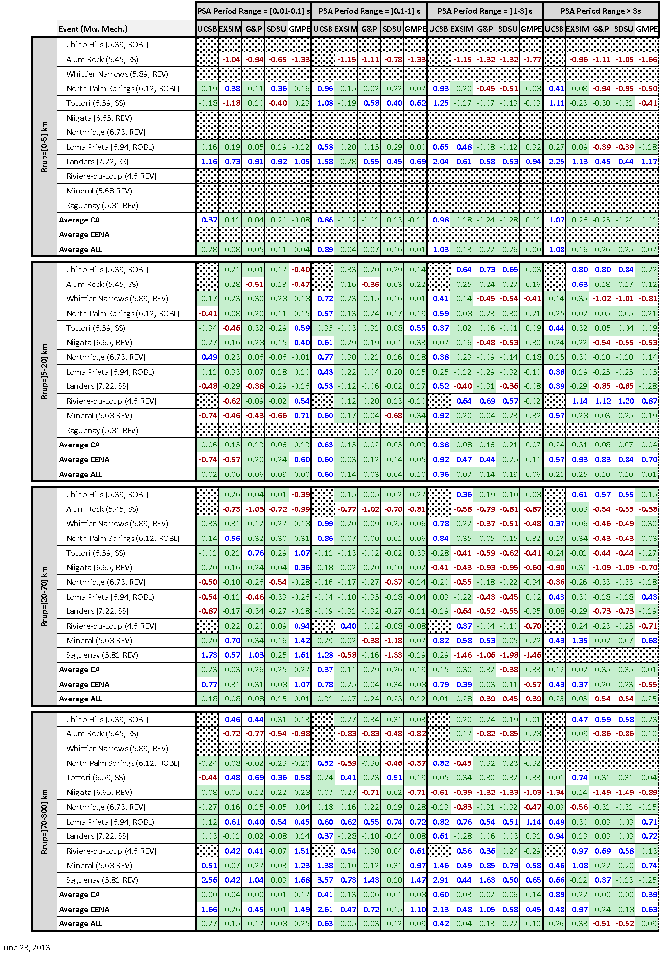
Figure S1. Mean bias using ln(data) – ln(simulation) residuals. Green indicates residual or bias is between ±0.35 ln units. Red numbers show values that are less than −0.35 (simulations overestimate observations), and blue numbers show values that are more than +0.35 (simulations underestimate observations). For details on the simulation methods (UCSB, EXSIM, G&P, SDSU, and GMPE), see the main article. Averages are listed for California (CA) and central and eastern North America (CENA), along with the average from all locations.
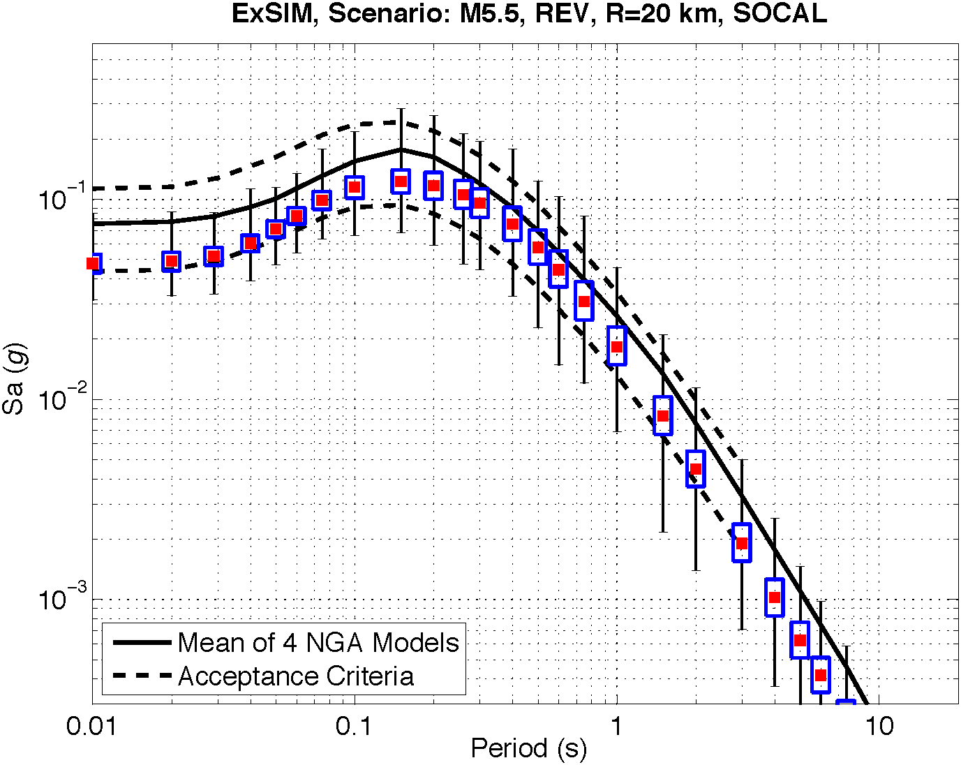
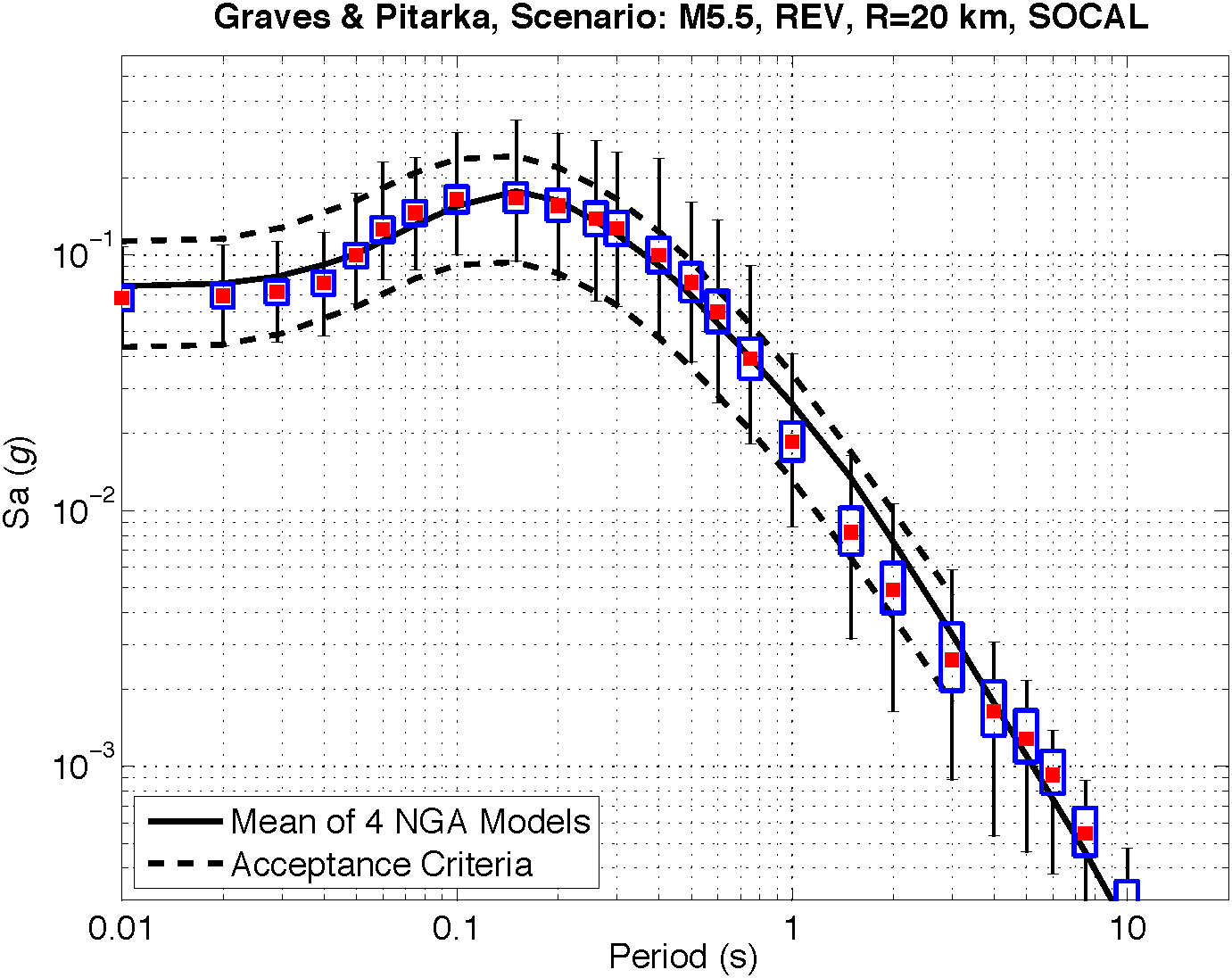
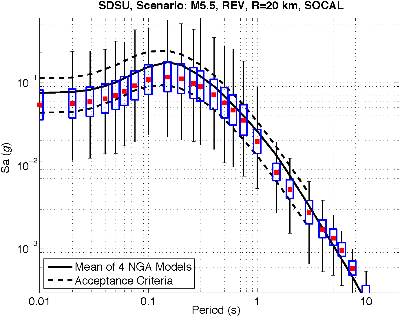
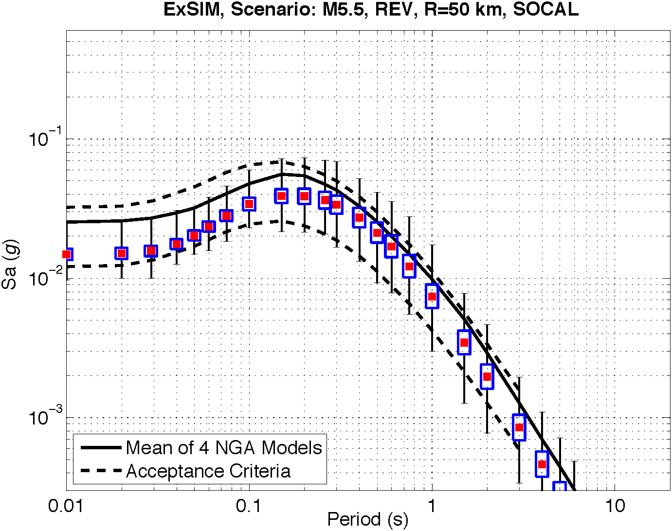
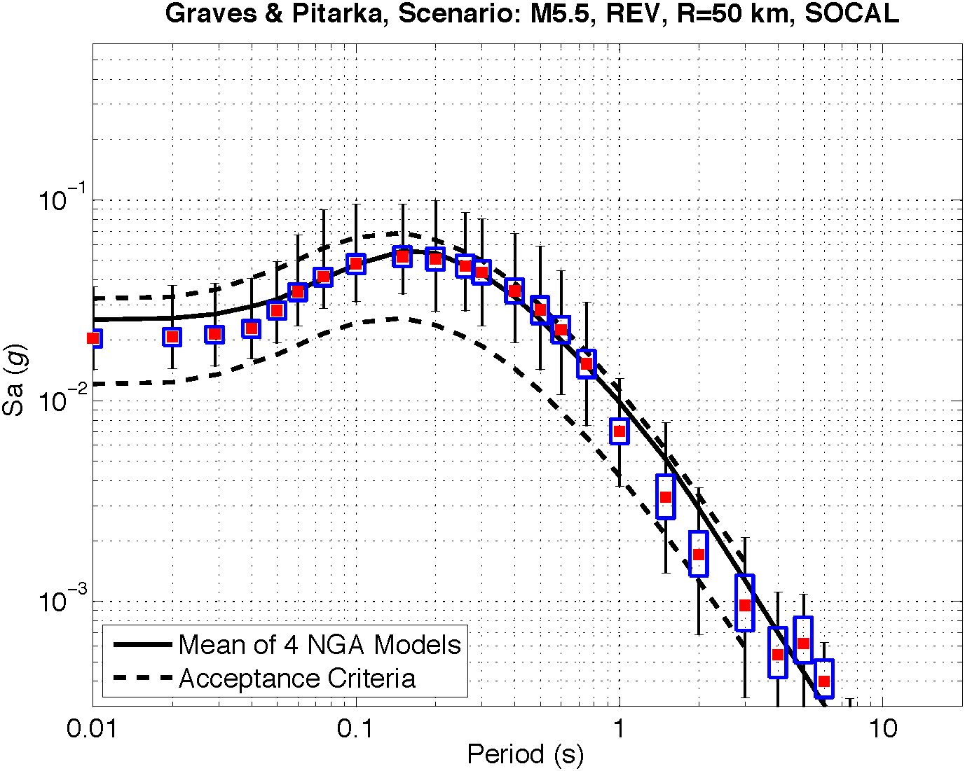
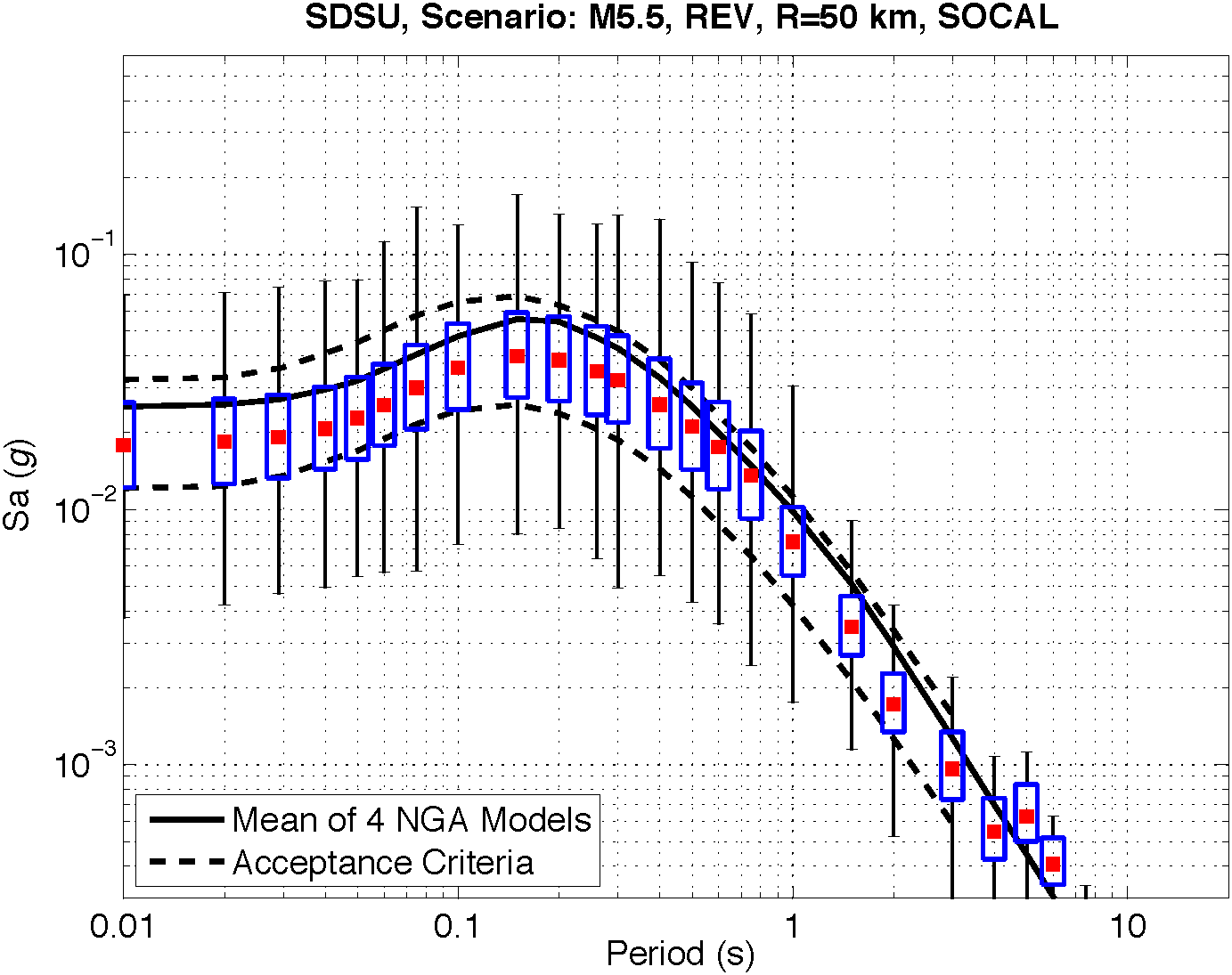
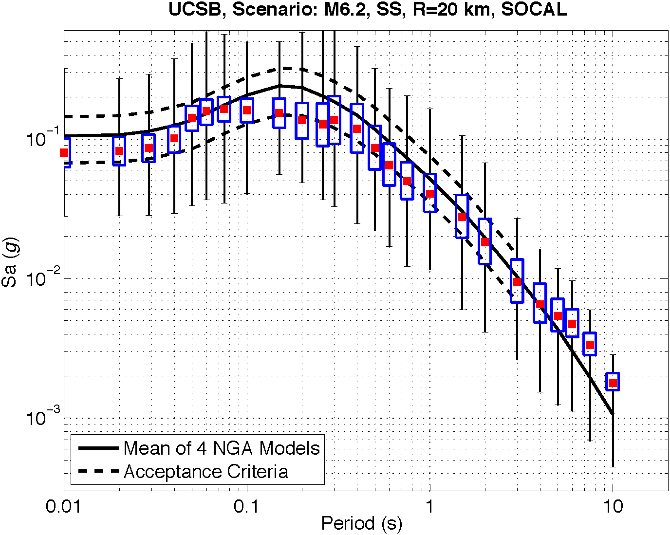
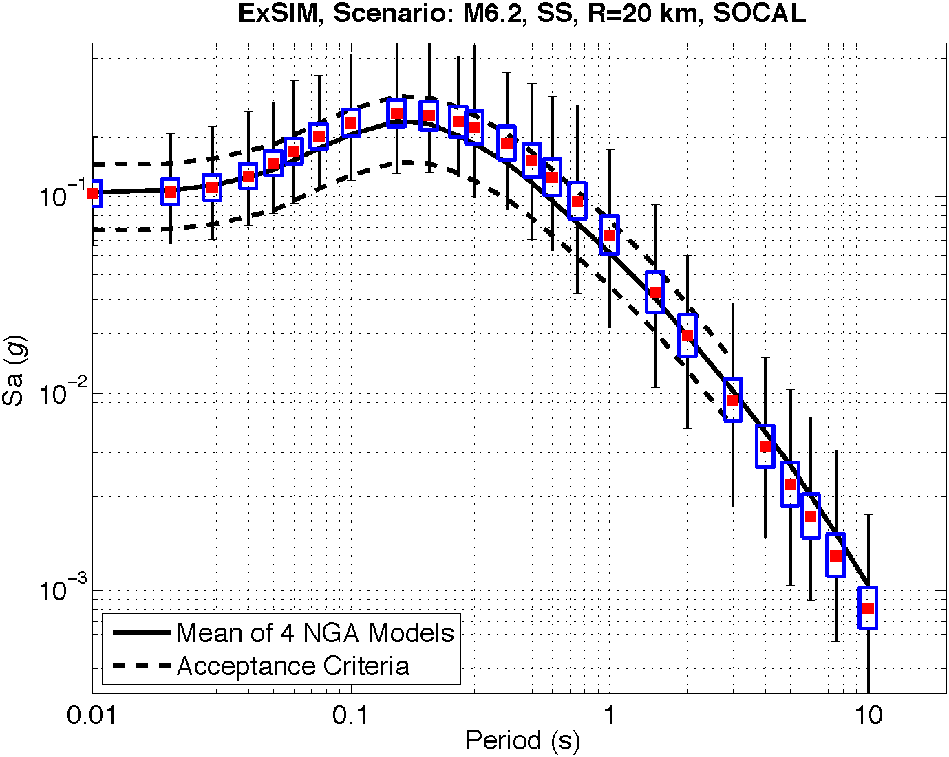
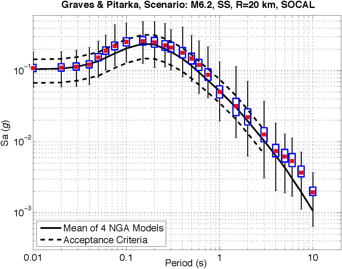
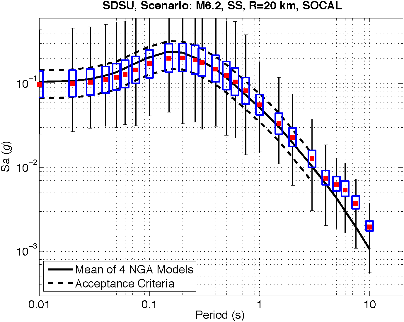
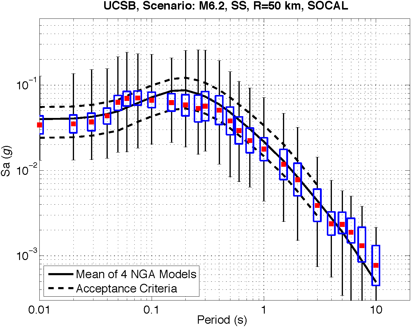
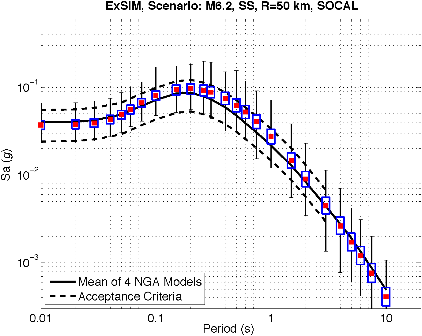
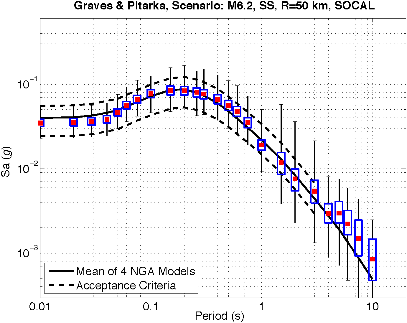
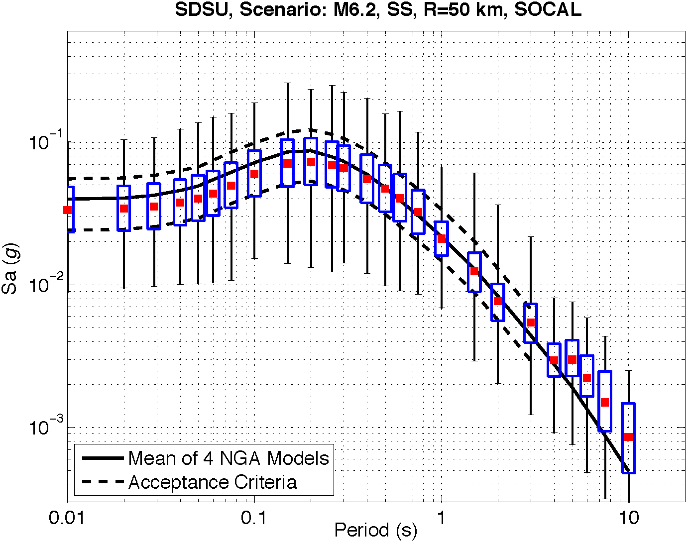
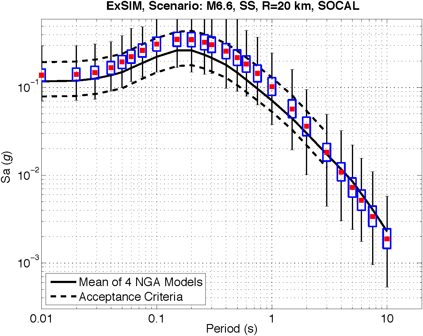
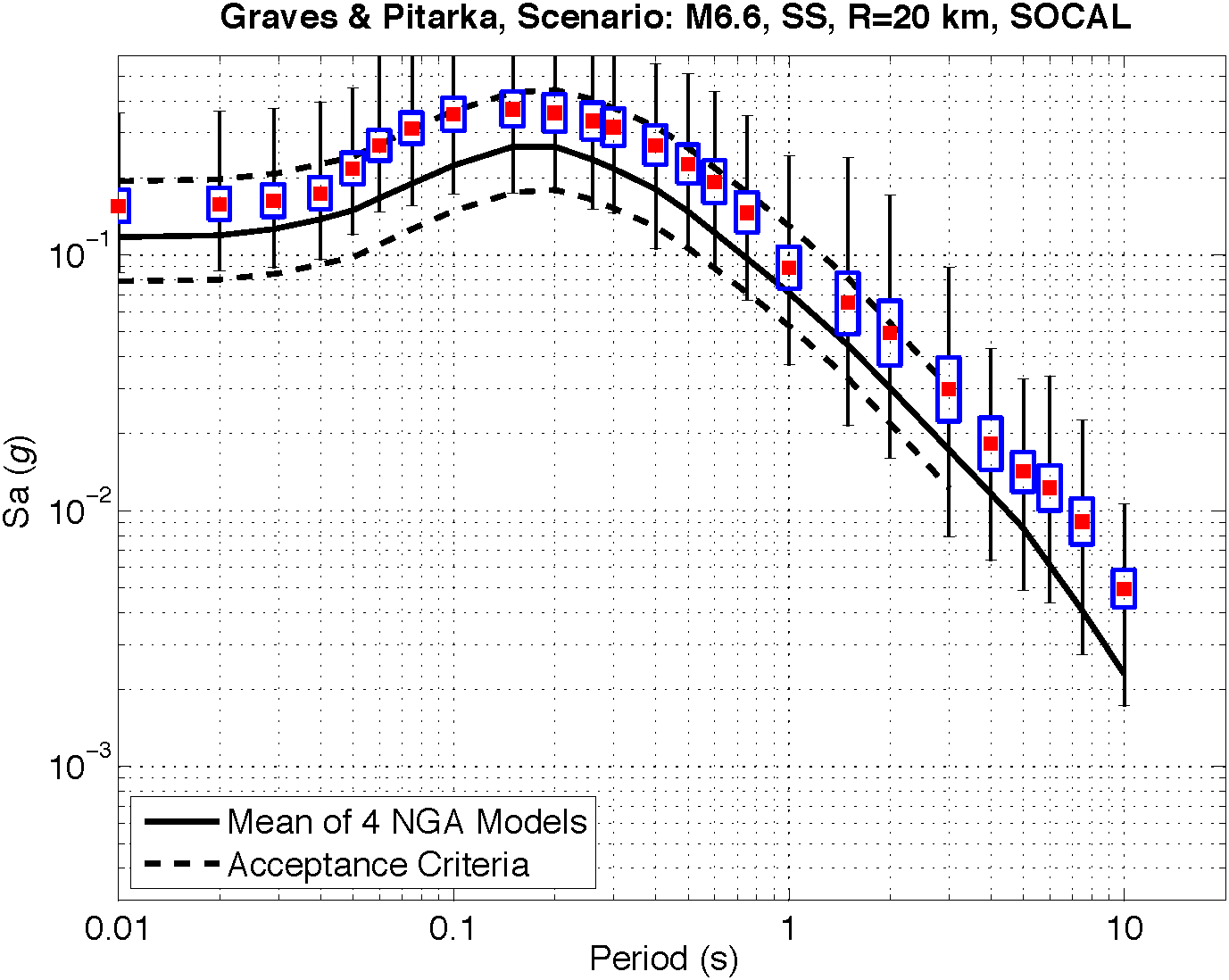
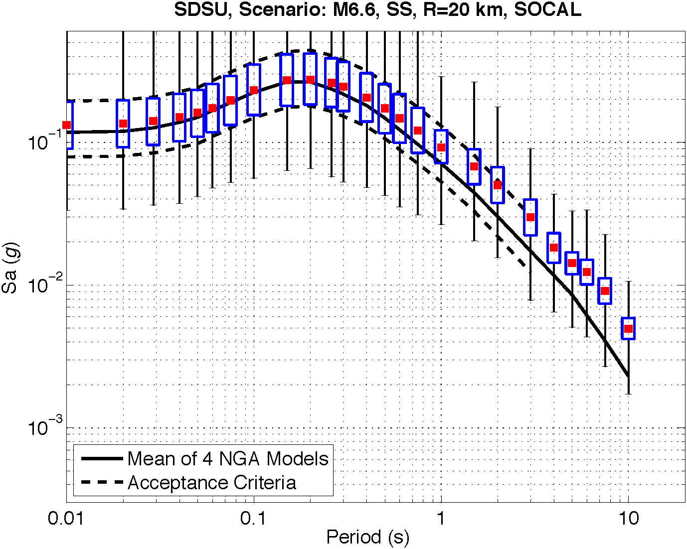
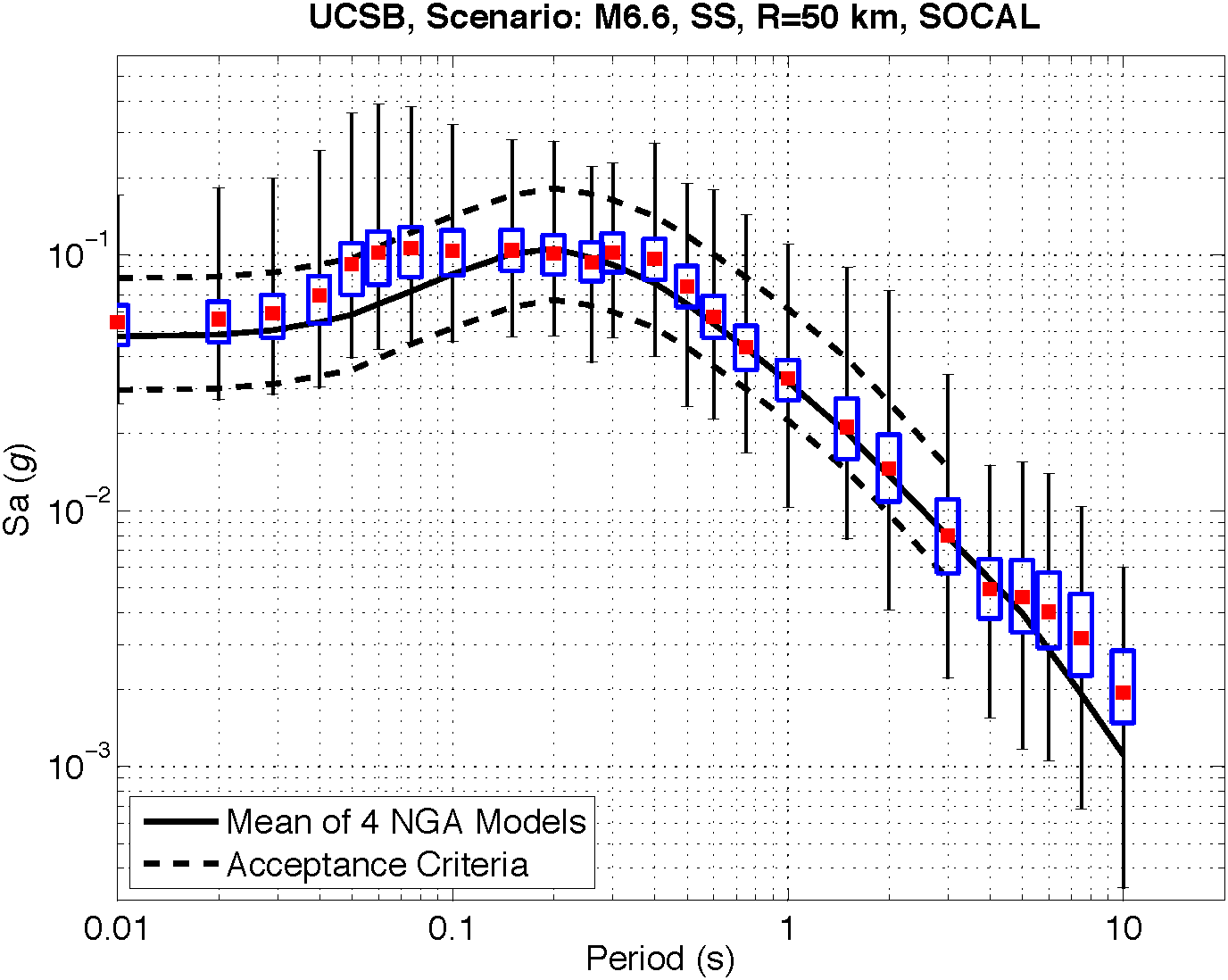
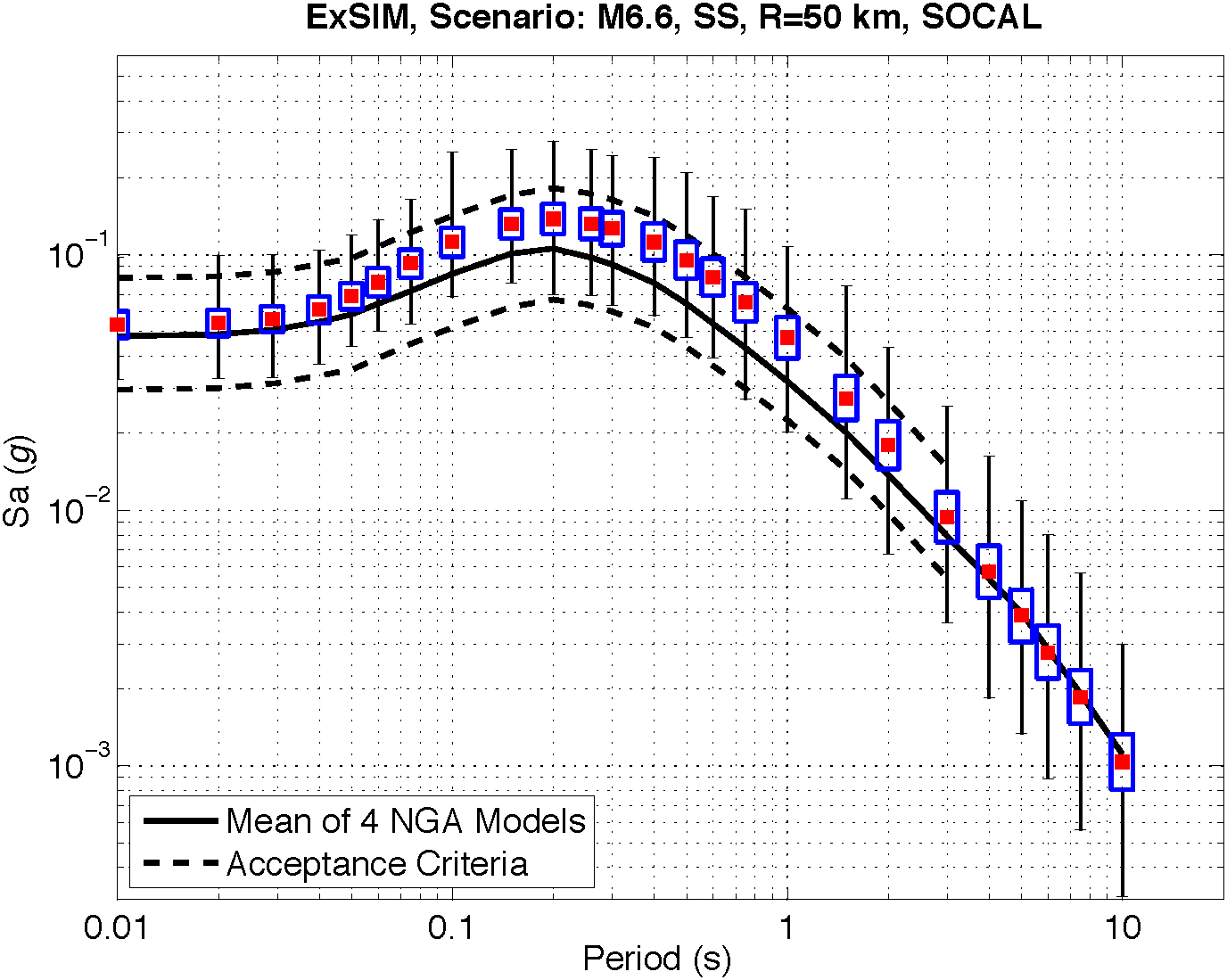
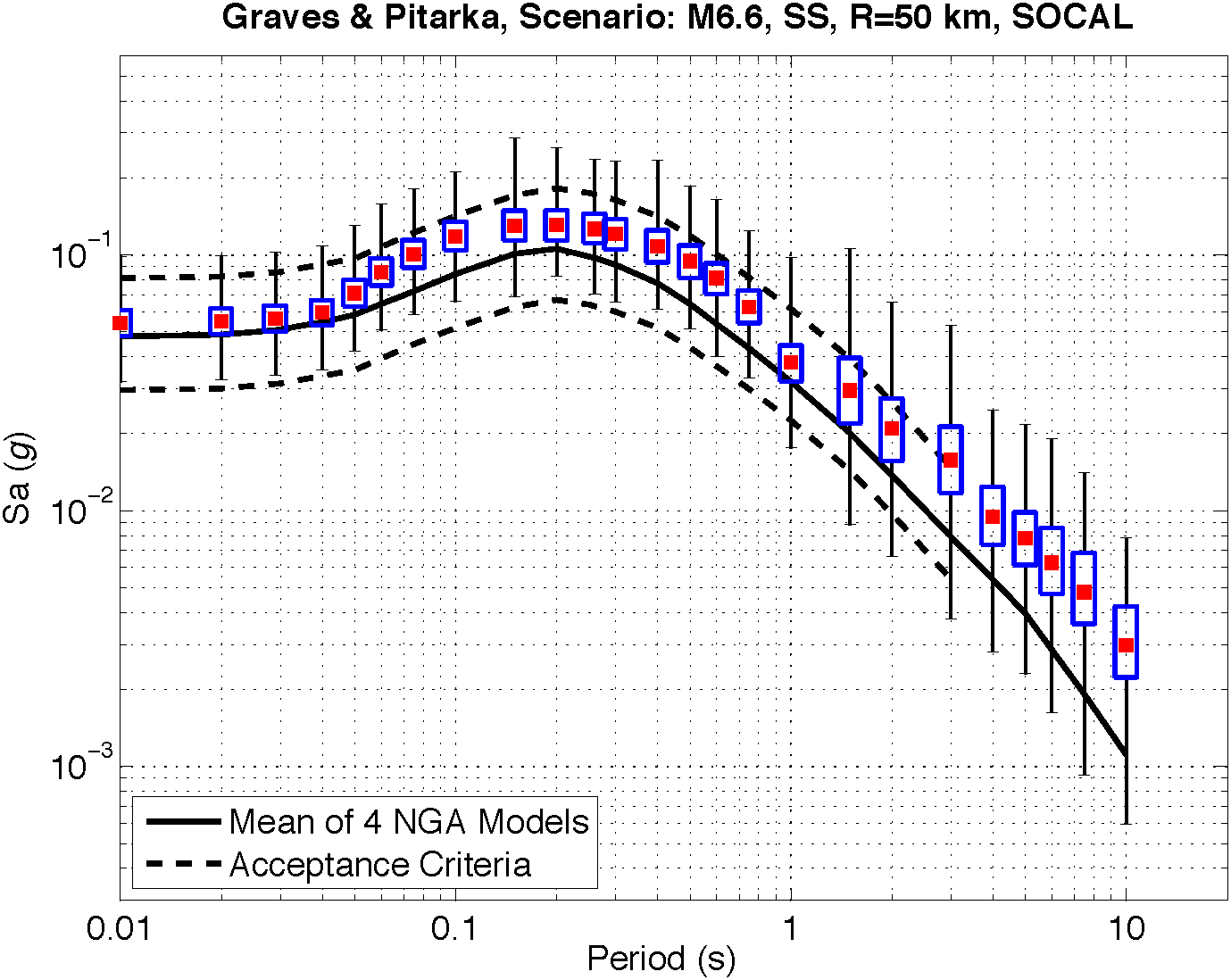
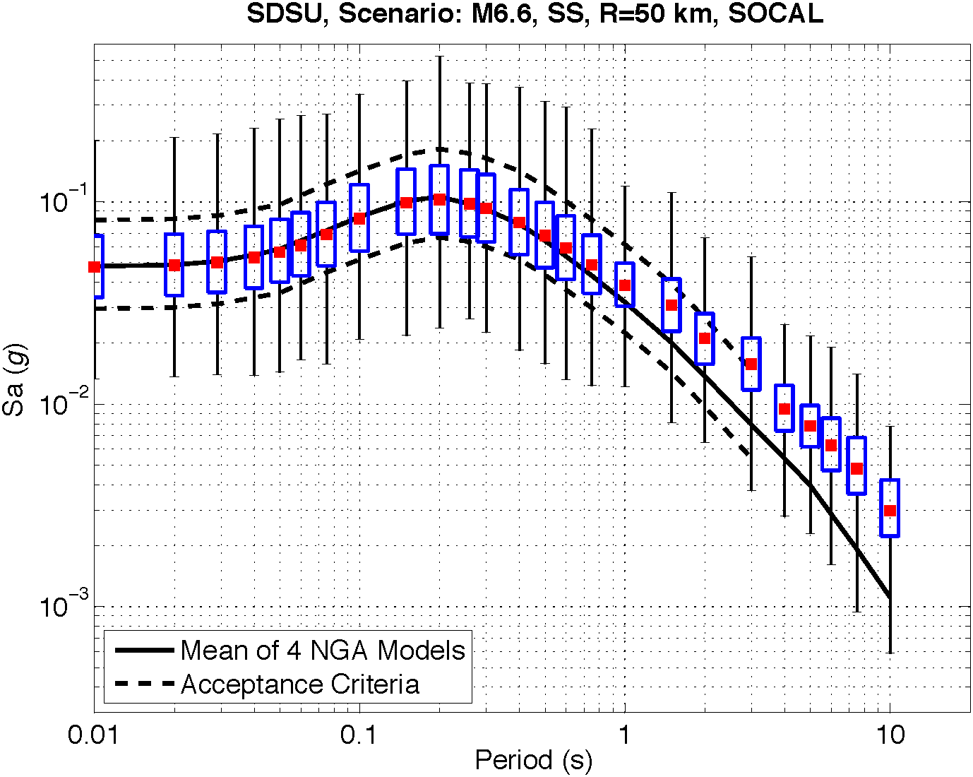
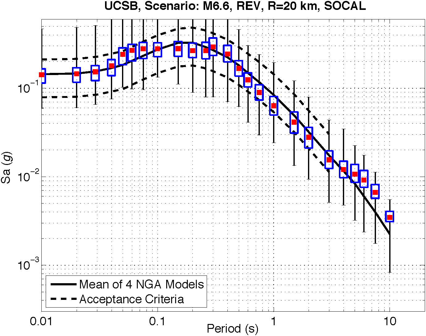
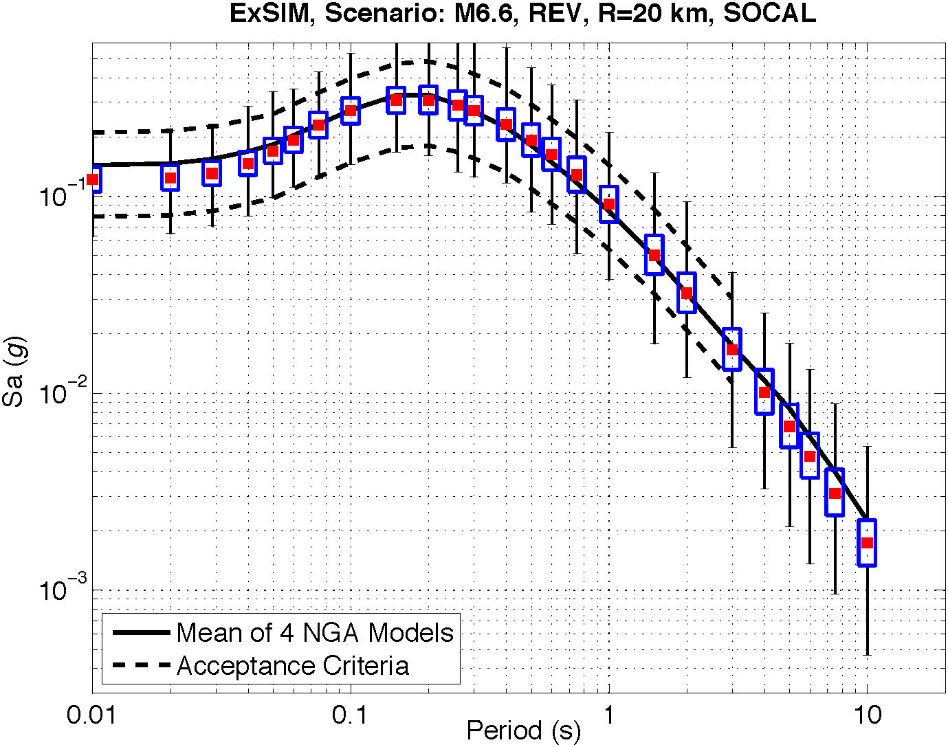
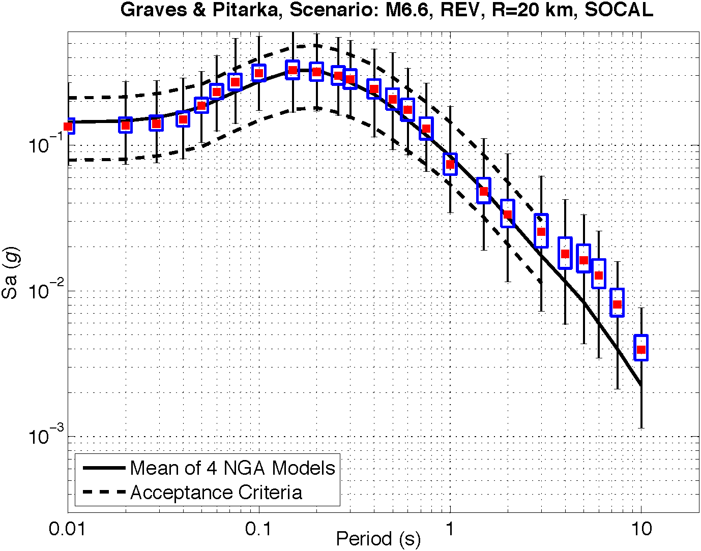
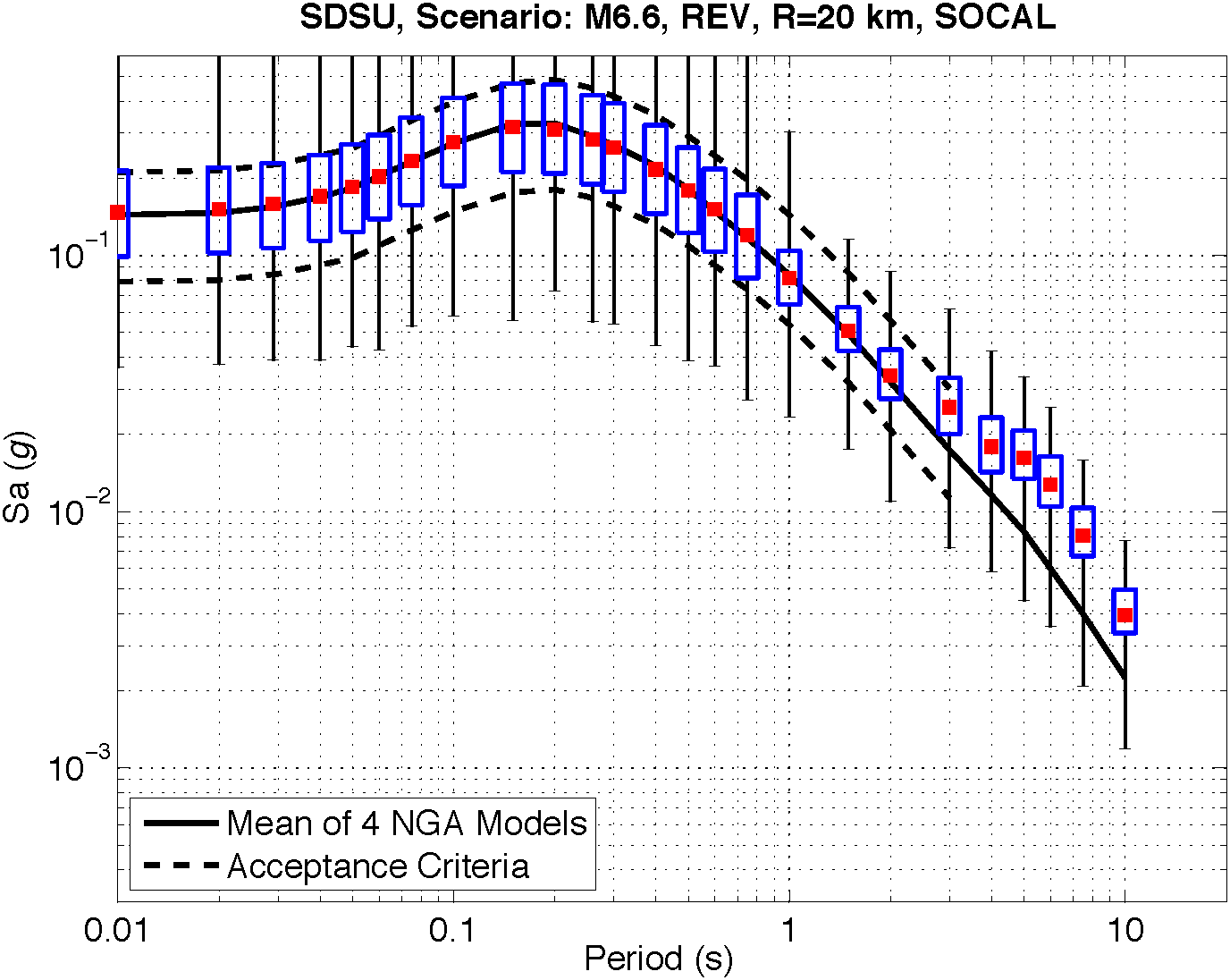
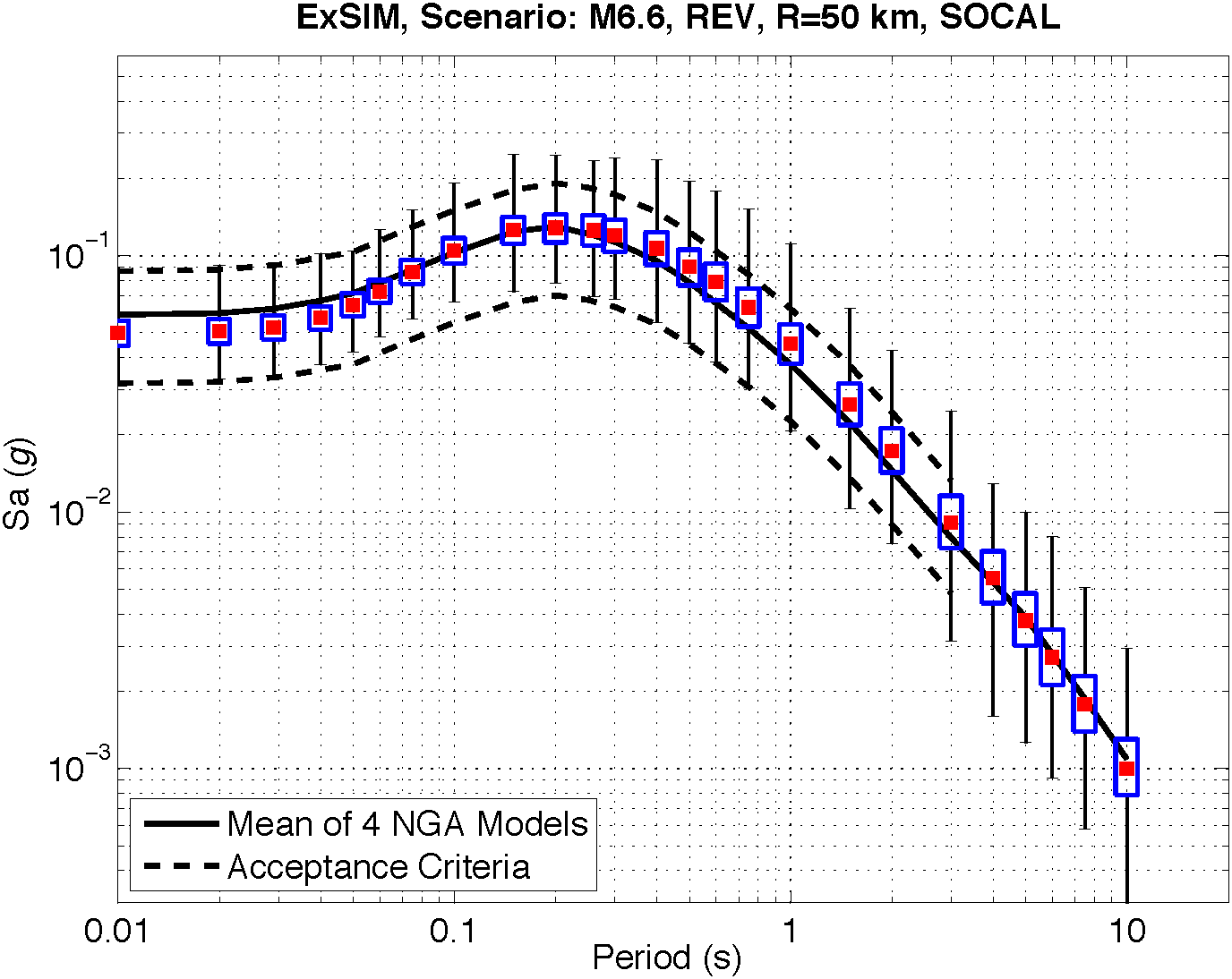
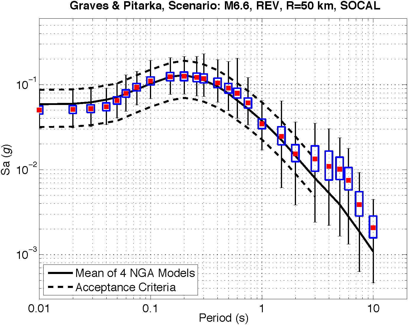
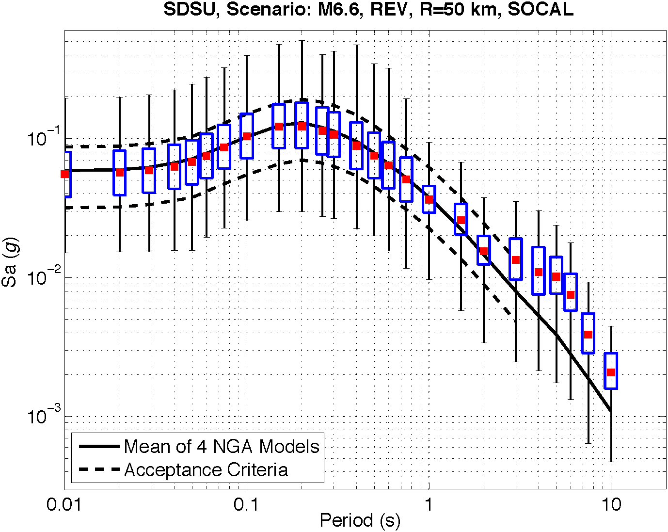
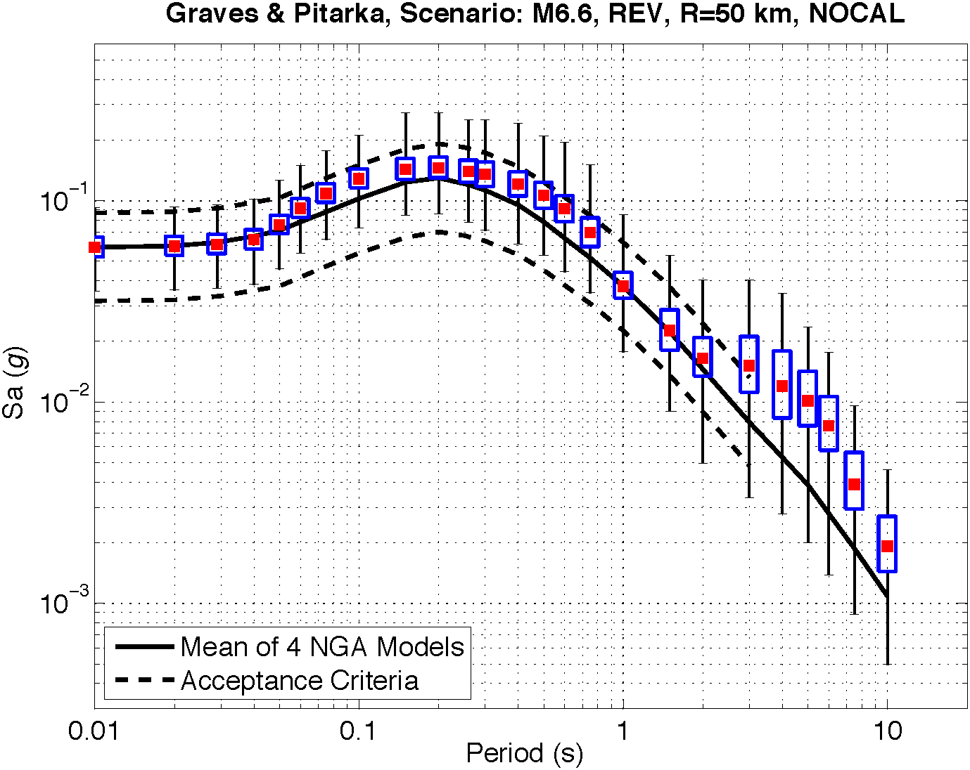
For Figures S2–S32, the red squares show the mean motion, the blue boxes the standard deviation, and the black bars the maximum range of simulated motions for 50 source realizations. The solid black line shows the mean from four NGA-West 1 (NGA-W1) GMPEs, and the dashed curves are the acceptance limits of the mean motions as described in the main article. The method and specific details of each scenario (magnitude, mechanism, distance [R] and velocity model used by the G&P, SDSU, and UCSB simulation methods [SOCAL or NOCAL] are indicated above each figure.
Figure S2. Comparison between EXSIM and Next Generation Attenuation (NGA) GMPE for an M 5.5 reverse mechanism at 20 km using SOCAL.
Figure S3. Comparison between G&P and NGA GMPE for an M 5.5 reverse mechanism at 20 km using SOCAL.
Figure S4. Comparison between SDSU and NGA GMPE for an M 5.5 reverse mechanism at 20 km using SOCAL.
Figure S5. Comparison between EXSIM and NGA GMPE for an M 5.5 reverse mechanism at 50 km using SOCAL.
Figure S6. Comparison between G&P and NGA GMPE for an M 5.5 reverse mechanism at 50 km using SOCAL.
Figure S7. Comparison between SDSU and NGA GMPE for an M5 .5 reverse mechanism at 50 km using SOCAL.
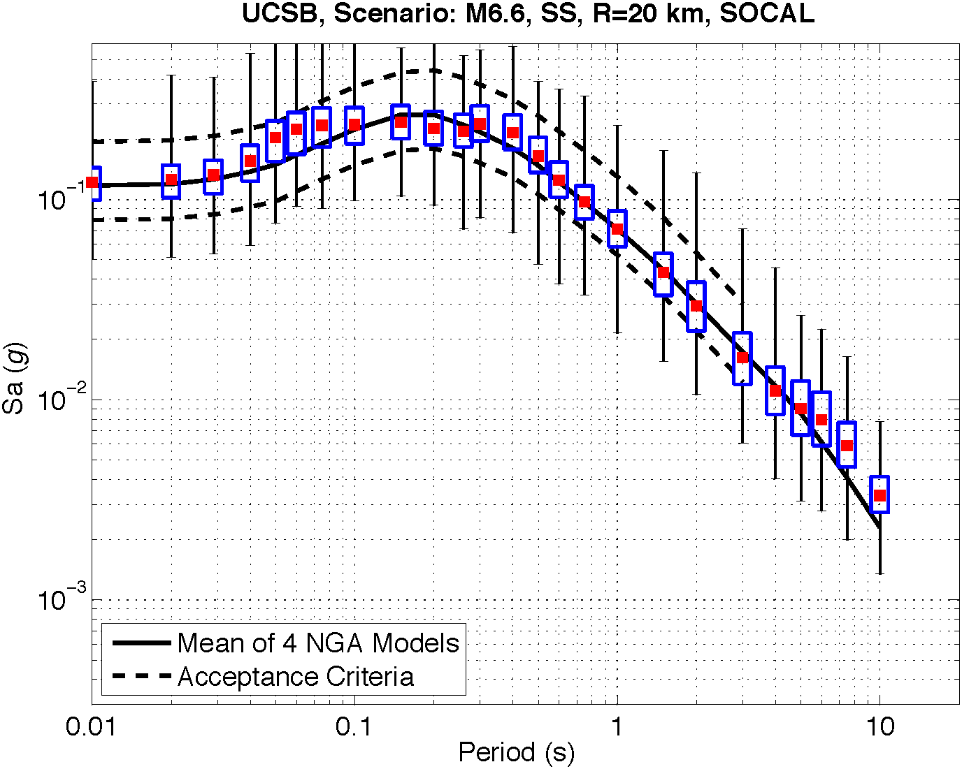
Figure S8. Comparison between UCSB and NGA GMPE for an M 6.2 strike-slip mechanism at 20 km using SOCAL.
Figure S9. Comparison between EXSIM and NGA GMPE for an M 6.2 strike-slip mechanism at 20 km using SOCAL.
Figure S10. Comparison between G&P and NGA GMPE for an M 6.2 strike-slip mechanism at 20 km using SOCAL.
Figure S11. Comparison between SDSU and NGA GMPE for an M 6.2 strike-slip mechanism at 20 km using SOCAL.
Figure S12. Comparison between UCSB and NGA GMPE for an M 6.2 strike-slip mechanism at 50 km using SOCAL.
Figure S13. Comparison between EXSIM and NGA GMPE for an M 6.2 strike-slip mechanism at 50 km using SOCAL.
Figure S14. Comparison between G&P and NGA GMPE for an M 6.2 strike-slip mechanism at 50 km using SOCAL.
Figure S15. Comparison between SDSU and NGA GMPE for an M 6.2 strike-slip mechanism at 50 km using SOCAL.
Figure S16. Comparison between UCSB and NGA GMPE for an M 6.6 strike-slip mechanism at 20 km. The red squares show the mean motion, the boxes the standard deviation, and the bars the maximum range of simulated motions for 50 source realizations. The black line shows the mean from four NGA-W1 GMPEs, and the dashed curves are the acceptance limits of the mean motions as described in the manuscript. SOCAL refers to the velocity model used by the G&P, SDSU and UCSB simulation methods.
Figure S17. Comparison between EXSIM and NGA GMPE for an M 6.6 strike-slip mechanism at 20 km using SOCAL.
Figure S18. Comparison between G&P and NGA GMPE for an M 6.6 strike-slip mechanism at 20 km using SOCAL.
Figure S19. Comparison between SDSU and NGA GMPE for an M 6.6 strike-slip mechanism at 20 km using SOCAL.
Figure S20. Comparison between UCSB and NGA GMPE for an M 6.6 strike-slip mechanism at 50 km using SOCAL.
Figure S21. Comparison between EXSIM and NGA GMPE for an M 6.6 strike-slip mechanism at 50 km using SOCAL.
Figure S22. Comparison between G&P and NGA GMPE for an M 6.6 strike-slip mechanism at 50 km using SOCAL.
Figure S23. Comparison between SDSU and NGA GMPE for an M 6.6 strike-slip mechanism at 50 km using SOCAL.
Figure S24. Comparison between UCSB and NGA GMPE for an M 6.6 reverse mechanism at 20 km using SOCAL.
Figure S25. Comparison between EXSIM and NGA GMPE for an M 6.6 reverse mechanism at 20 km using SOCAL.
Figure S26. Comparison between G&P and NGA GMPE for an M 6.6 reverse mechanism at 20 km using SOCAL.
Figure S27. Comparison between SDSU and NGA GMPE for an M 6.6 reverse mechanism at 20 km using SOCAL.
Figure S28. Comparison between UCSB and NGA GMPE for an M 6.6 reverse mechanism at 50 km using SOCAL.
Figure S29. Comparison between EXSIM and NGA GMPE for an M 6.6 reverse mechanism at 50 km using SOCAL.
Figure S30. Comparison between G&P and NGA GMPE for an M 6.6 reverse mechanism at 50 km using SOCAL.
Figure S31. Comparison between SDSU and NGA GMPE for an M 6.6 reverse mechanism at 50 km using SOCAL.
Figure S32. Comparison between G&P and NGA GMPE for an M 6.6 reverse mechanism at 50 km using NOCAL. A comparison of Figure S29 and S31 shows that there is some difference in the simulation results in the intermediate period range due to the choice of velocity model.
[ Back ]