This electronic supplement includes supporting figures and a 3D ground-motion simulation animation.
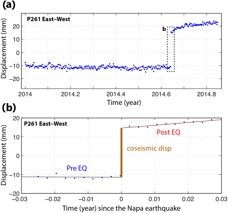
Figure S1. An example of continuous Global Positioning System (cGPS) coseismic displacement estimation from daily solutions. (a) Time series since 1 January 2014 in the east–west component at station P261. (b) The east–west component of P261 10 days before (blue dots) and after (red dots) the South Napa earthquake (EQ); the two black lines are the least-squares fitting to the time series. The estimated coseismic displacement (disp) is the difference between the two black lines at time t = 0.
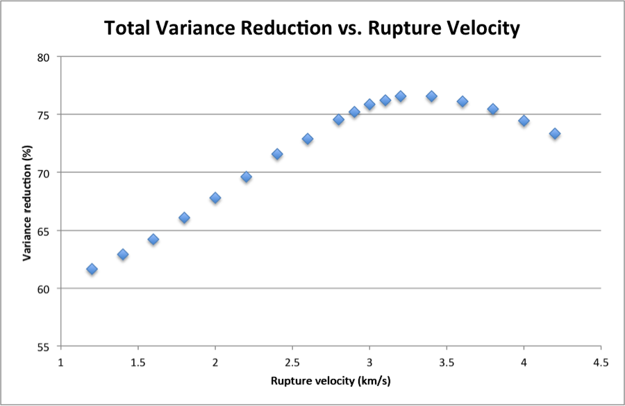
Figure S2. Composite variance reduction, computed as the average of the variance reduction goodness of fit for the three data sets is compared to rupture velocity.
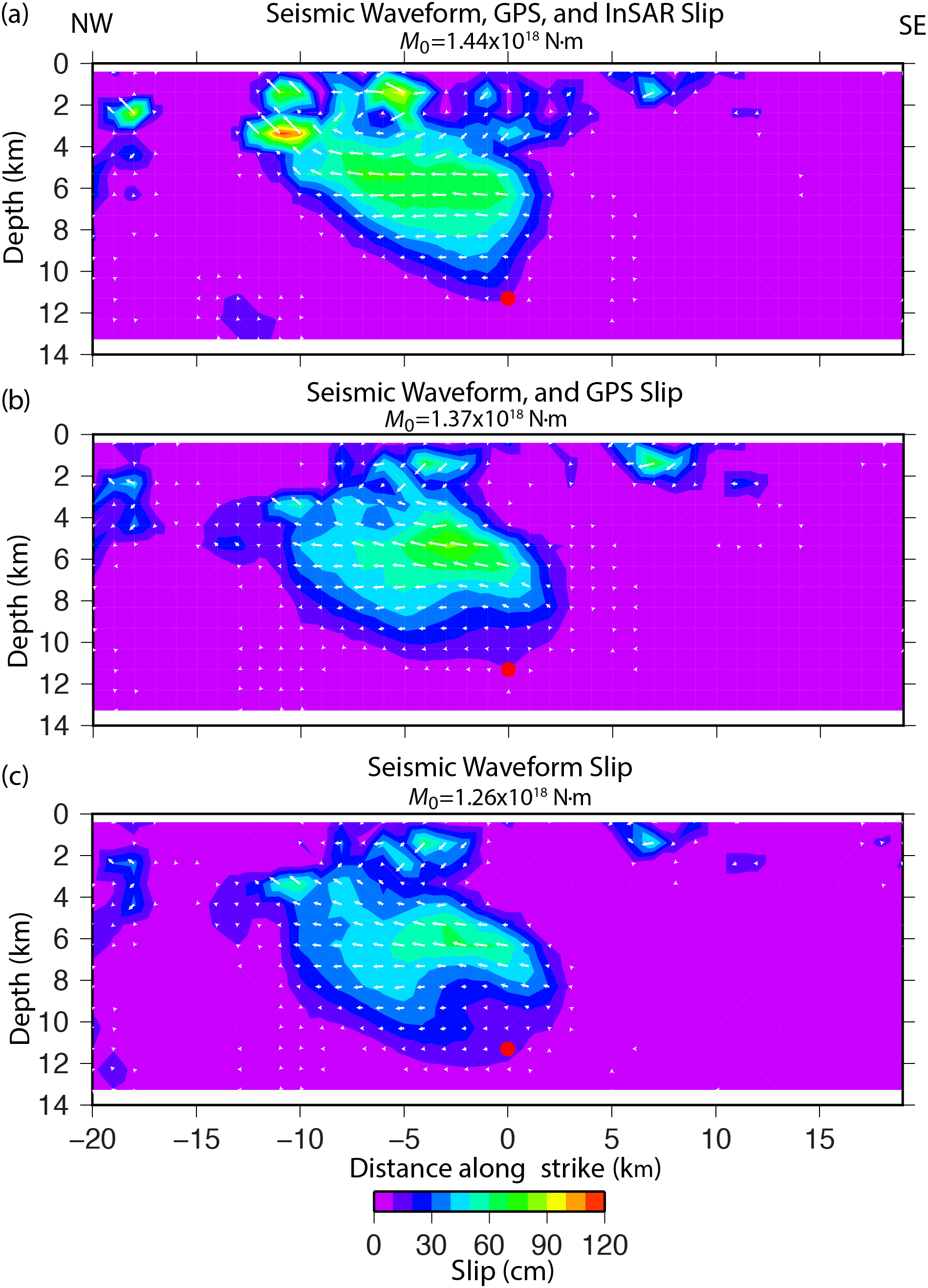
Figure S3. Comparision of (a) joint seismic waveform, GPS, and Interferometric Synthetic Aperture Radar (InSAR); (b) joint seismic waveform and GPS; and (c) seismic-waveform-only, for finite-source slip models. The white arrows indicate the slip direction, and the red circle shows the hypocenter.
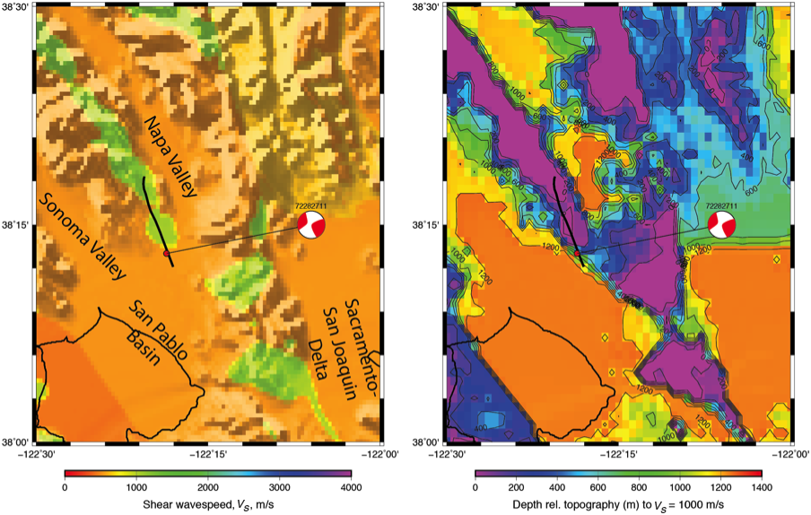
Figure S4. Geologic and 3D seismic structure near the South Napa earthquake, showing (left) geographic features, low resolution topography, and surface shear wavespeed (color scale) and (right) depth relative to the surface for the shear wavespeed of 1000 m/s, which roughly delineates the basin depth. Also shown in both panels is the surface rupture, the Northern California Seismic System (NCSS) epicenter and the Berkeley Seismological Laboratory moment tensor.
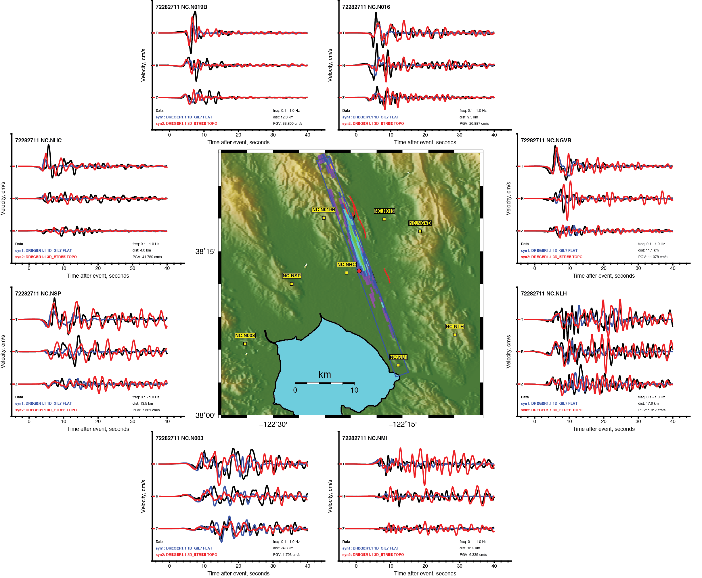
Figure S5. Waveform comparisons for the Mw 6.0 South Napa mainshock and map showing surface projection of the slip (same color scale as Figure S3), fault surface (blue box), surface rupture (black and red lines), and station locations. The waveform comparison panels show the observed (black) and synthetic waveforms (blue for GIL7 1D model and red for the USGS 3D model) filtered 0.1–1.0 Hz and displayed as transverse, radial (relative to the NCSS location), and vertical components.
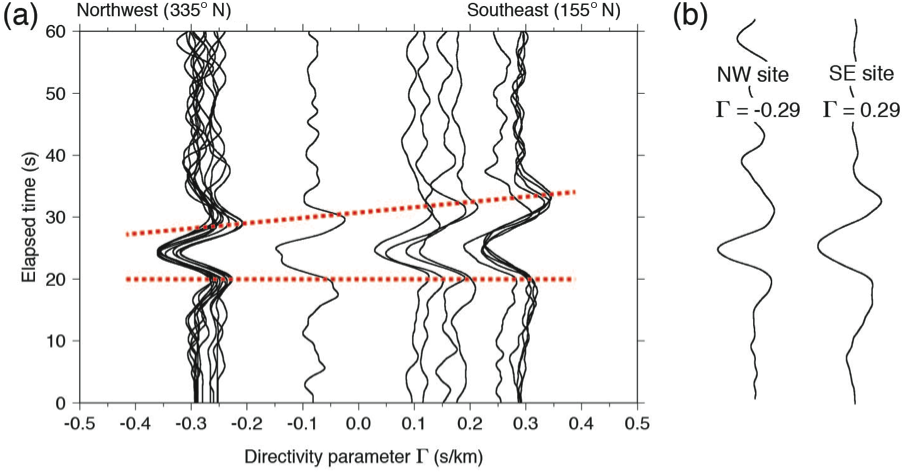
Figure S6. (a) Moment rate functions for the 2014 Mw 6.0 South Napa earthquake plotted as a function of directivity parameter Γ, assuming the rupture azimuth at 155° N with the phase velocity of 3.4 km/s. Moment rate functions are aligned by the onset of the pulse. A negative value of Γ indicates station azimuth along the northwest rupture direction. Note that a 0.1 Hz highpass filter was applied to suppress high-frequency noise. (b) Two selected moment rate functions from stations with positive and negative Γ.
Download/View: Animation S1 [h.264-encoded MP4; ~14.5 MB]. This animation compares a ground motion simulation for our kinematic finite-fault model using both (left) a 1D model (GIL7, Stidham et al., 1999) and (right) the U.S. Geological Survey 3D velocity model (USGS, 2014). The animation shows the magnitude of ground velocity and was computed with Lawrence Livermore National Laboratory’s SW4 code.
Petersson, N. A., and B. Sjogreen (2013). User’s guide to SW4, version 1.0, Lawrence Livermore National Laboratory Tech. Rept. LLNL-SM-642292, 114 pp.
Stidham, C., M. Antolik, D. Dreger, S. Larsen, and B. Romanowicz (1999). Three-dimensional structure influences on the strong-motion wavefield of the 1989 Loma Prieta earthquake, Bull. Seismol. Soc. Am. 89, 1184–1202.
United States Geologic Survey (2014). 3D Geologic and Seismic Velocity Models of the San Francisco Bay Region, http://earthquake.usgs.gov/data/3dgeologic/, (last accessed December 2014).
[ Back ]