This electronic supplement contains figures of waveform fits, predicted interferograms and surface displacement, and time-varying cumulative slip.
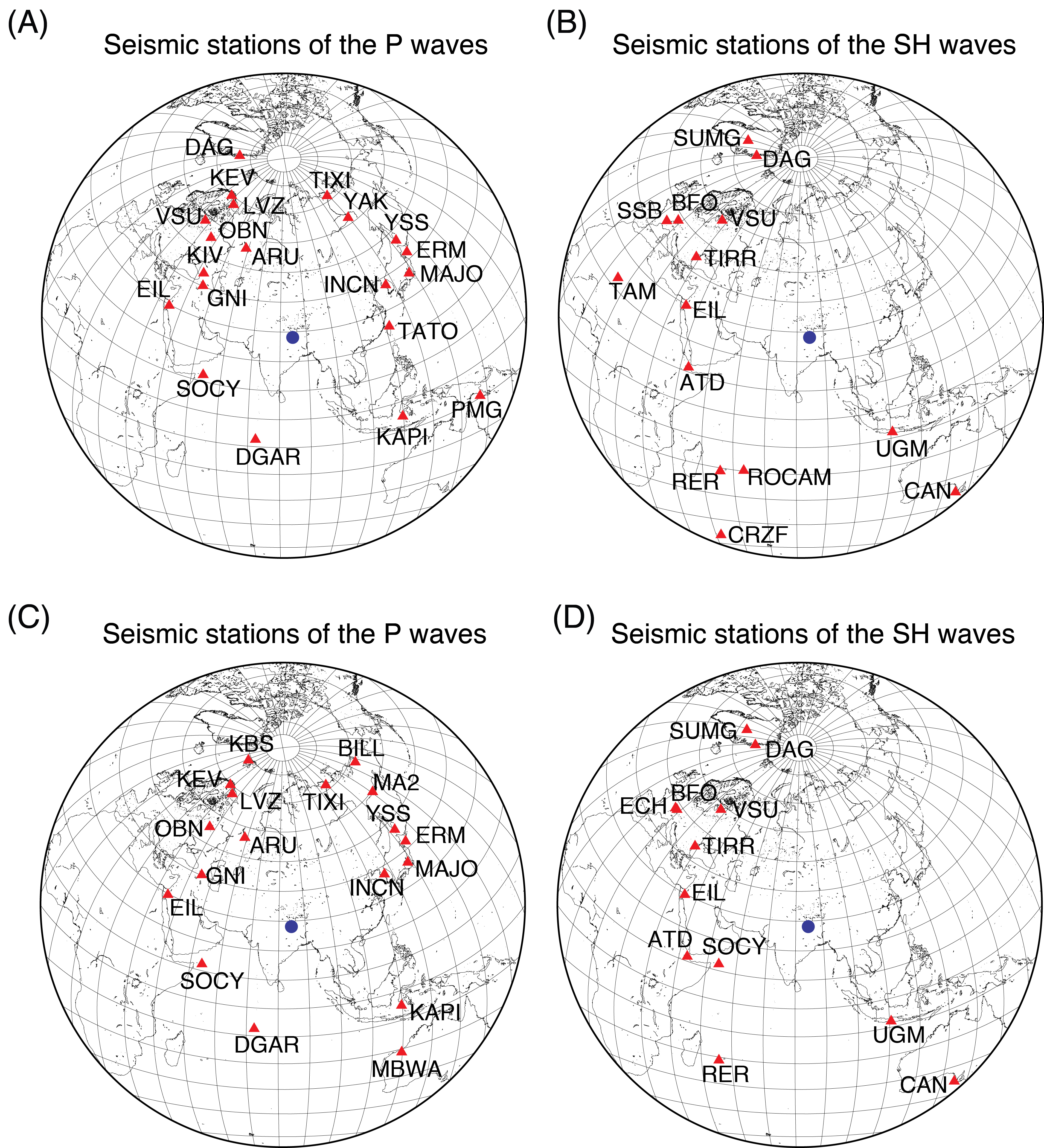
Figure S1 shows the distribution of seismic stations from which we used teleseismic data.
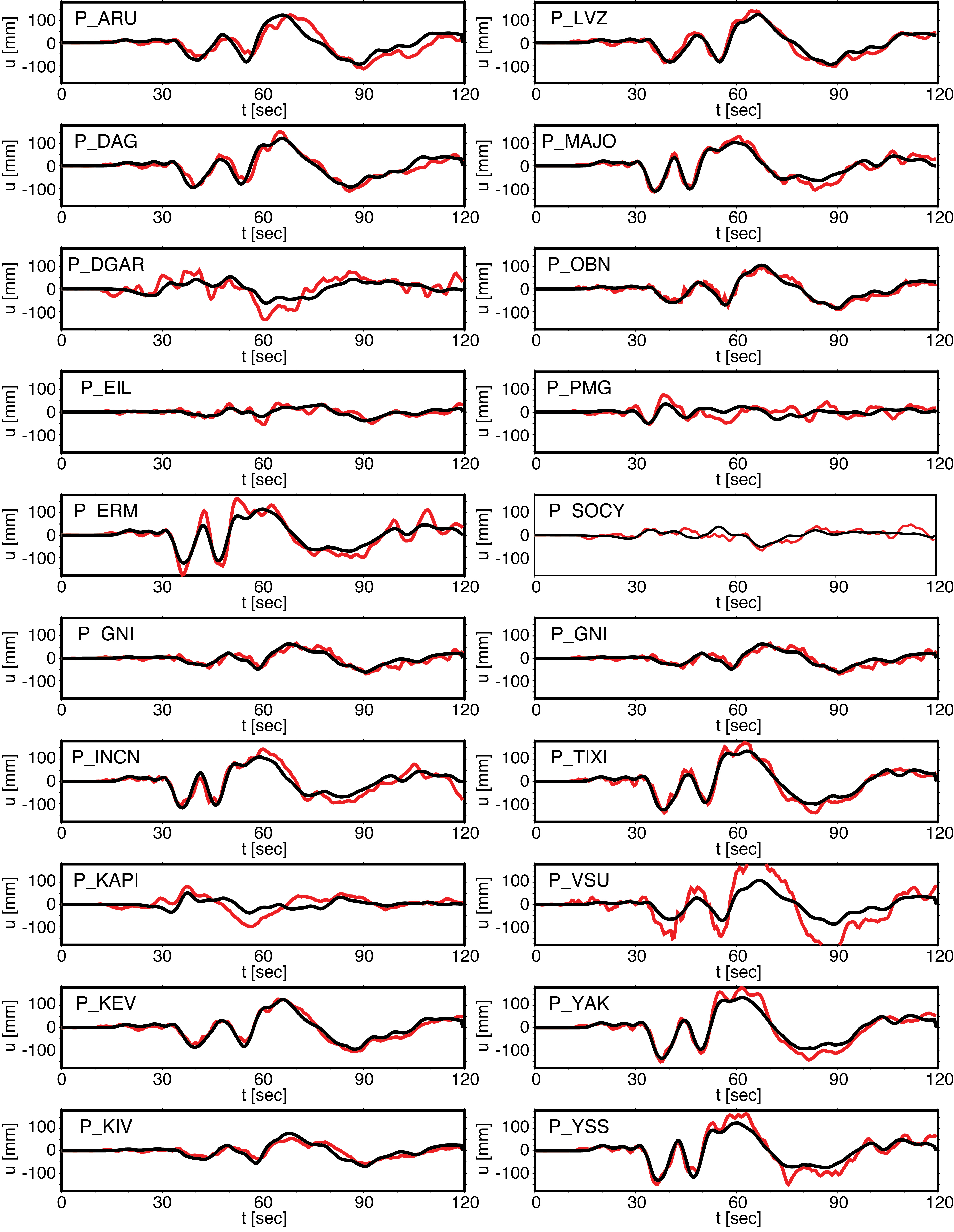
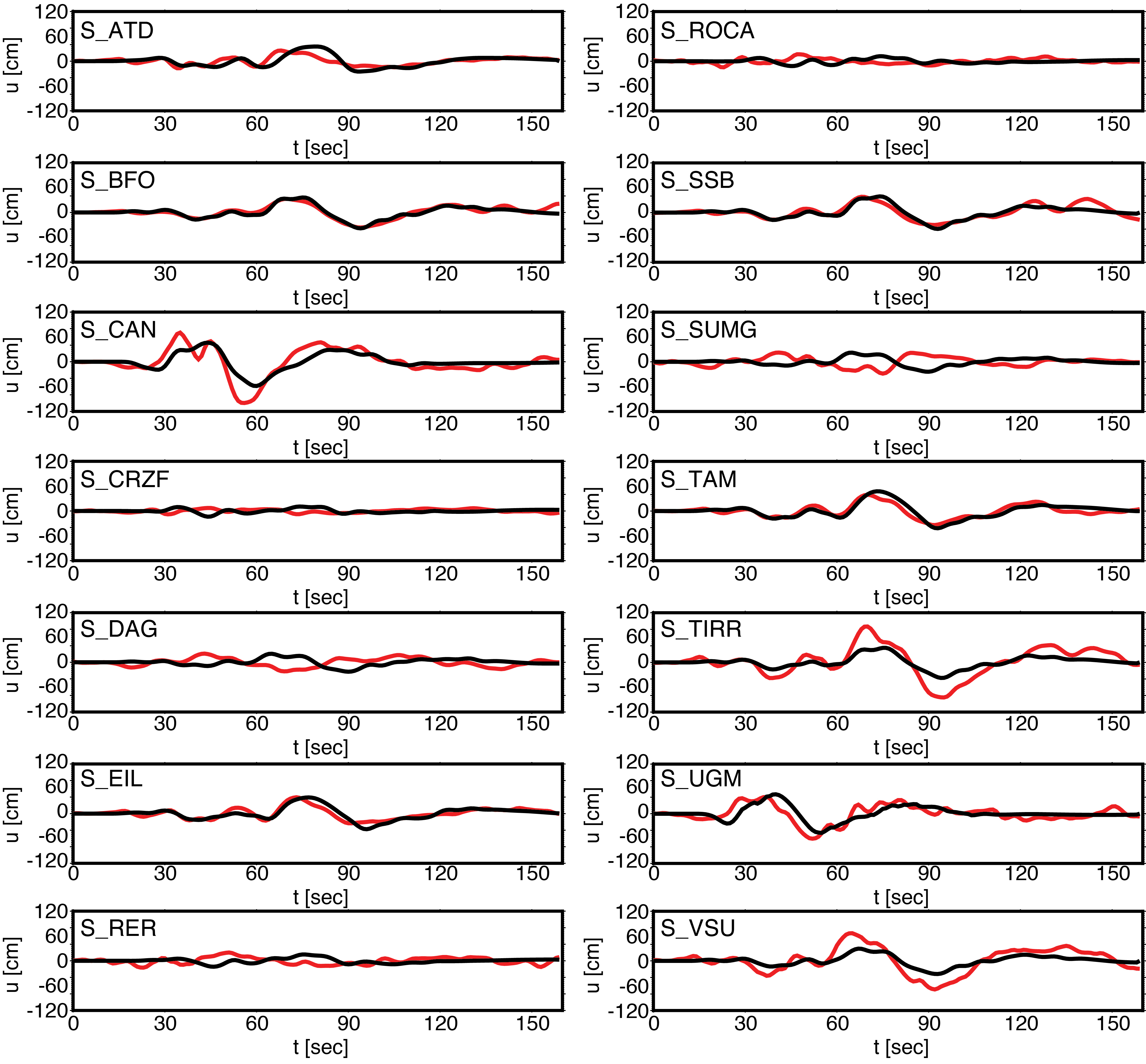
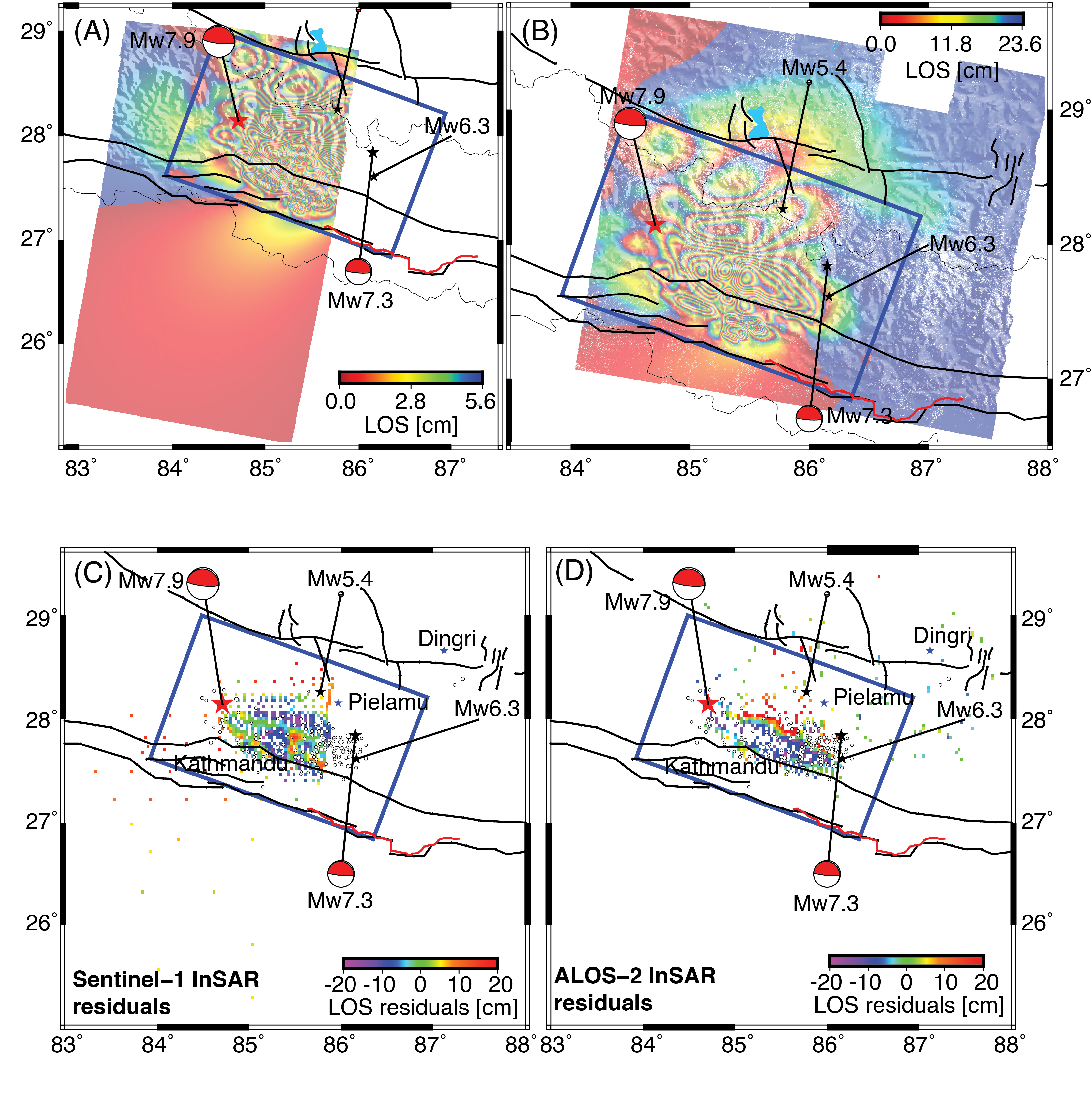
Teleseismic waveforms and the predictions of the waveforms from the final joint Gorkha slip model are shown in Figures S2 and S3. Figure S4 shows the predicted and residual Sentinel-1 and ALOS-2 interferograms.
Figure S5 depicts the spatiotemporal slip in the Kodari earthquake, showing cumulative slip in discrete time windows (snapshots of the kinematic slip model). Figure S6 also shows the source time function of the Kodari slip model. Teleseismic waveforms and the predictions of the waveforms from the final joint Kodari slip model are shown in Figures S6 and S7. Figure S7 shows the observed, predicted, and residual ALOS-2 interferograms.
Figure S9 depicts the spatiotemporal slip in the Gorkha earthquake inferred when we assigned equal weight to the GPS and InSAR data. A comparison of Figure S9 with the preferred slip model shown in Figure 4 of the main article indicates that, although changing the weights does affect minor details of the inferred slip, the main features we interpret in this paper are similar between the two. Specifically, the coseismic slip breaks into two main slip patches east of the hypocenter, one up-dip and one down-dip with smaller slip. Additionally, the delayed coseismic slip in the center of the up-dip patch, with the initial coseismic slip skipping over this patch, is seen in both models.
Figure S1. (a) and (b) Distributions of the seismic stations from which we obtained the P and SH teleseismic waveforms used to constrain the slip in the Gorkha earthquake. (c) and (d) Distribution of seismic stations from which we obtained the teleseismic waveforms used to constrain the slip in the Kodari earthquake.
Figure S2. Teleseismic P waveforms of the Gorkha earthquake used to constrain the slip model (red), and the teleseismic waveforms predicted by the Gorkha slip model determined by jointly inverting all of the available data (black).
Figure S3. Observed (red) and predicted (black) teleseismic S waveforms of the Gorkha earthquake and joint slip model, respectively.
Figure S4. Predicted interferograms corresponding to (a) the Sentinal-1 and (b) the ALOS-2 interferograms from the European Space Agency InSARap program and Lindsey et al. (2015), respectively, and residuals between (c) the predicted and (d) the observed interferograms. Predicted interferograms are shown at the full field of the interferogram footprint for ease of comparison with Figure 1, and the residuals are shown at the decimated points used in the inversion. Focal mechanisms and epicenter (red star) of the Gorkha and Kodari earthquakes and two larger aftershocks (black stars) are shown, as are the surface traces of the main faults in the Himalayan thrust fault system (black lines) and the assumed surface trace of the Nepal–Bihar earthquake (red line). The blue rectangle is the surface projection of the outline of the model fault model used in the slip inversion, and black dots are the subfault centers.
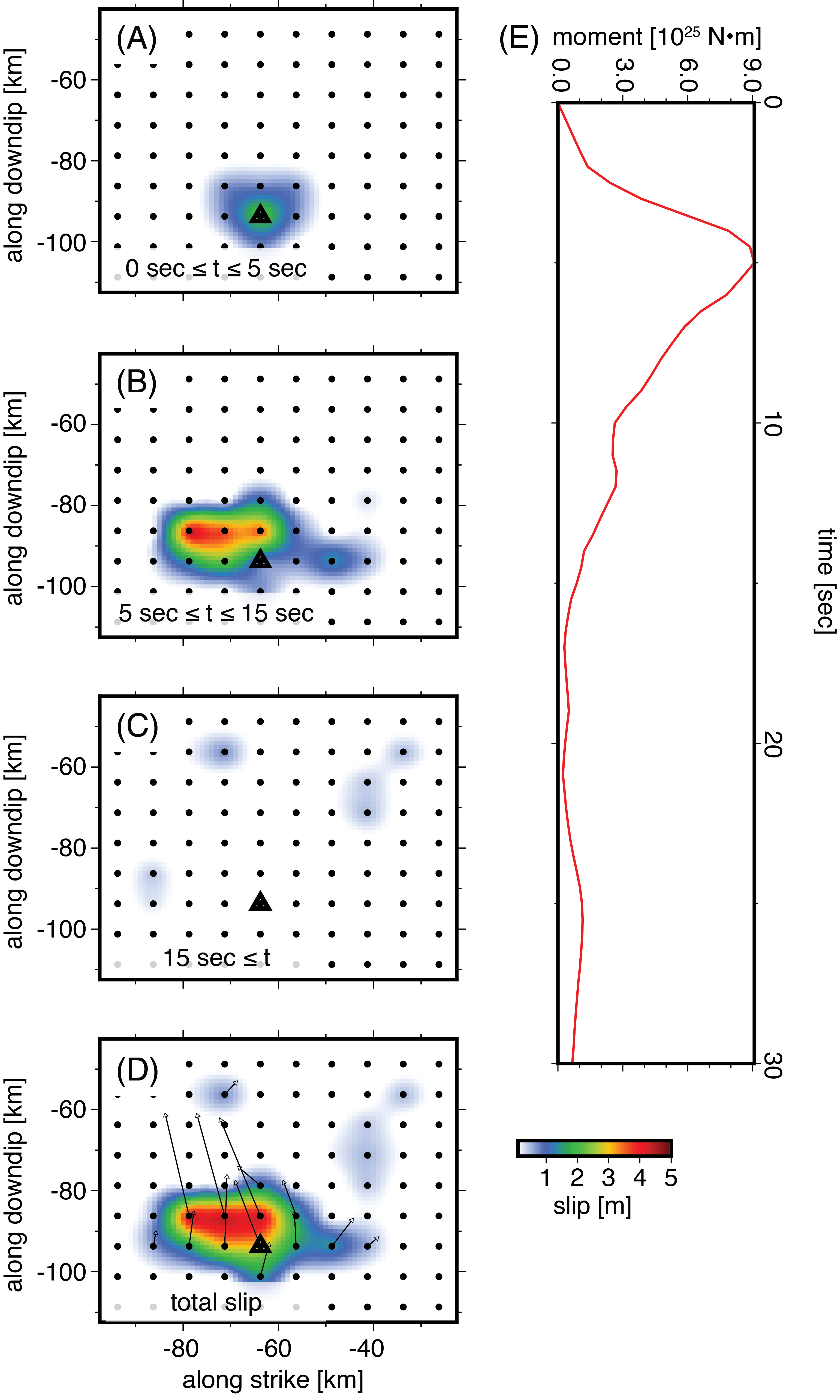
Figure S5. Cumulative slip in the joint Kodari slip model within (a) the first 5 s, (b) the next 10 seconds, (c) the last 15 seconds, and (d) over the entire earthquake. The black triangle is the hypocenter of the Kodari earthquake, and black circles are the centers of the subfaults. (e) Source time function of the slip model for the Kodari earthquake, determined from inverting all data jointly.
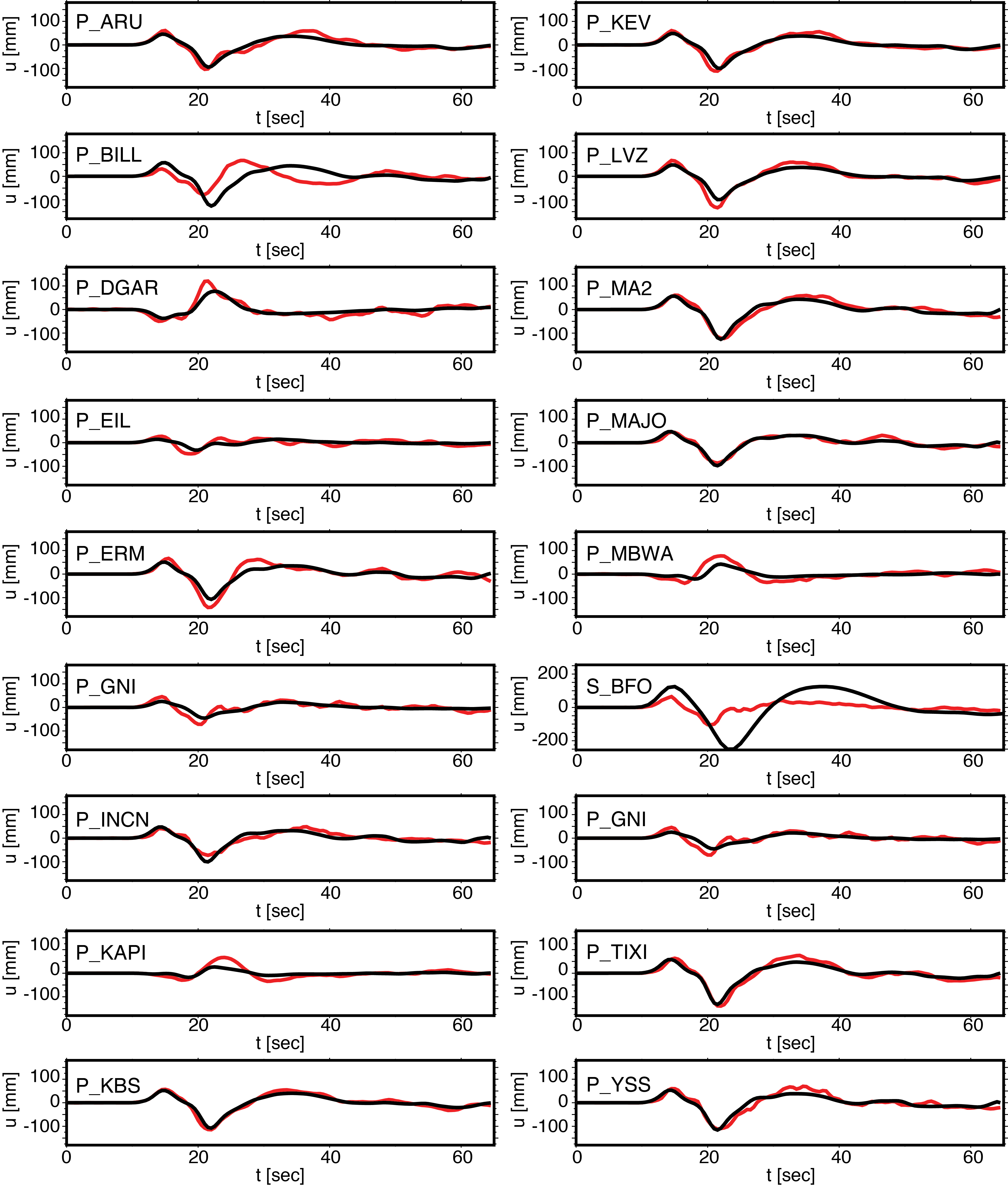
Figure S6. Observed (red) and predicted (black) teleseismic P waveforms of the Kodari earthquake and joint slip model, respectively.
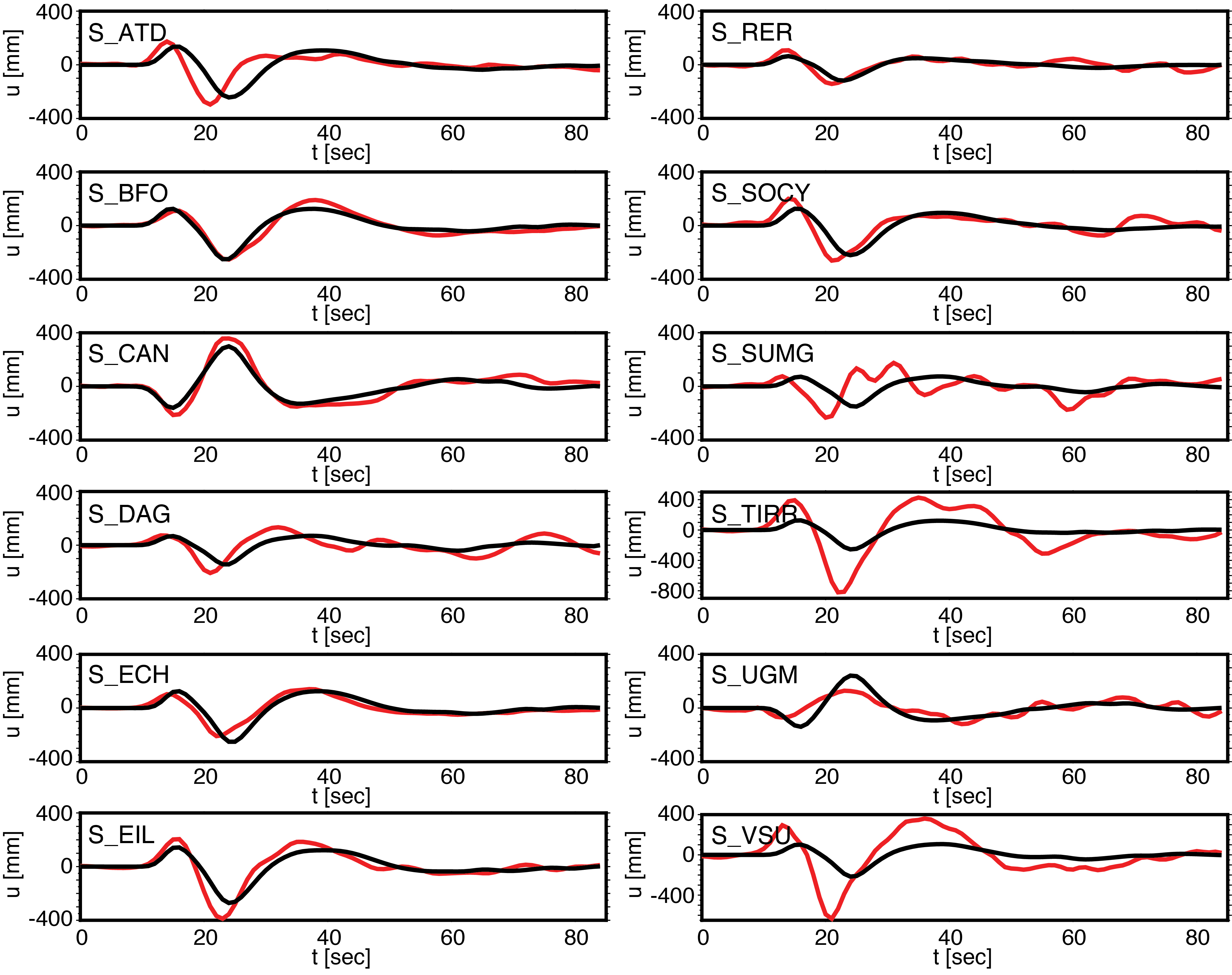
Figure S7. Observed (red) and predicted (black) teleseismic S waveforms of the Kodari earthquake and joint slip model, respectively.
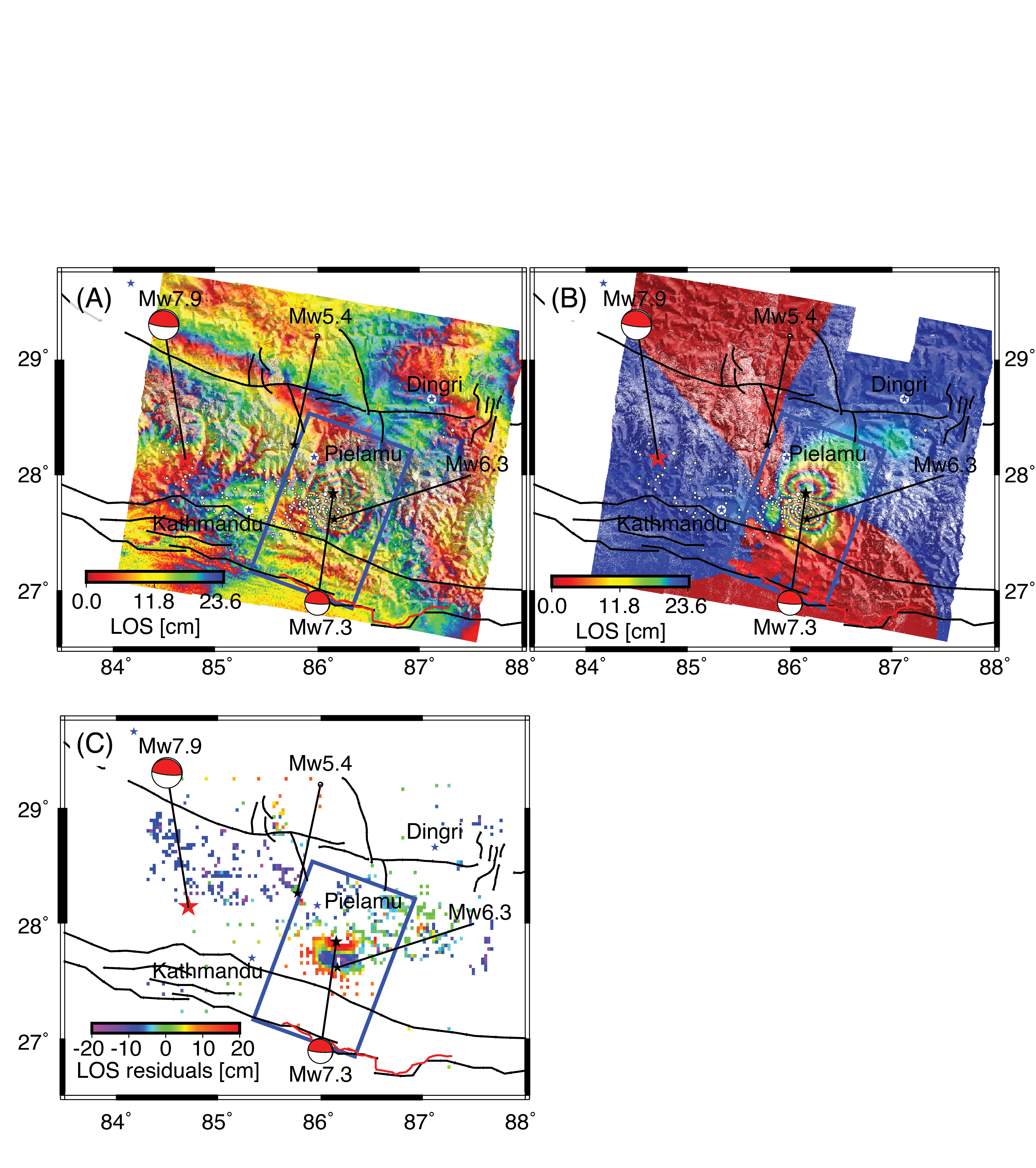
Figure S8. (a) ALOS-2 interferogram showing line-of-sight (LOS) surface displacements due to the Kodari earthquake (Lindsey et al., 2015). The blue rectangle is the surface projection of the fault outline in the slip model. Other symbols are as in Figure S3. (b) Predicted interferogram corresponding to (a). (c) Residual between the predicted and observed interferograms. Predicted interferograms are shown at the full field of the interferogram footprint, and the residuals are shown at the decimated points used in the inversion.
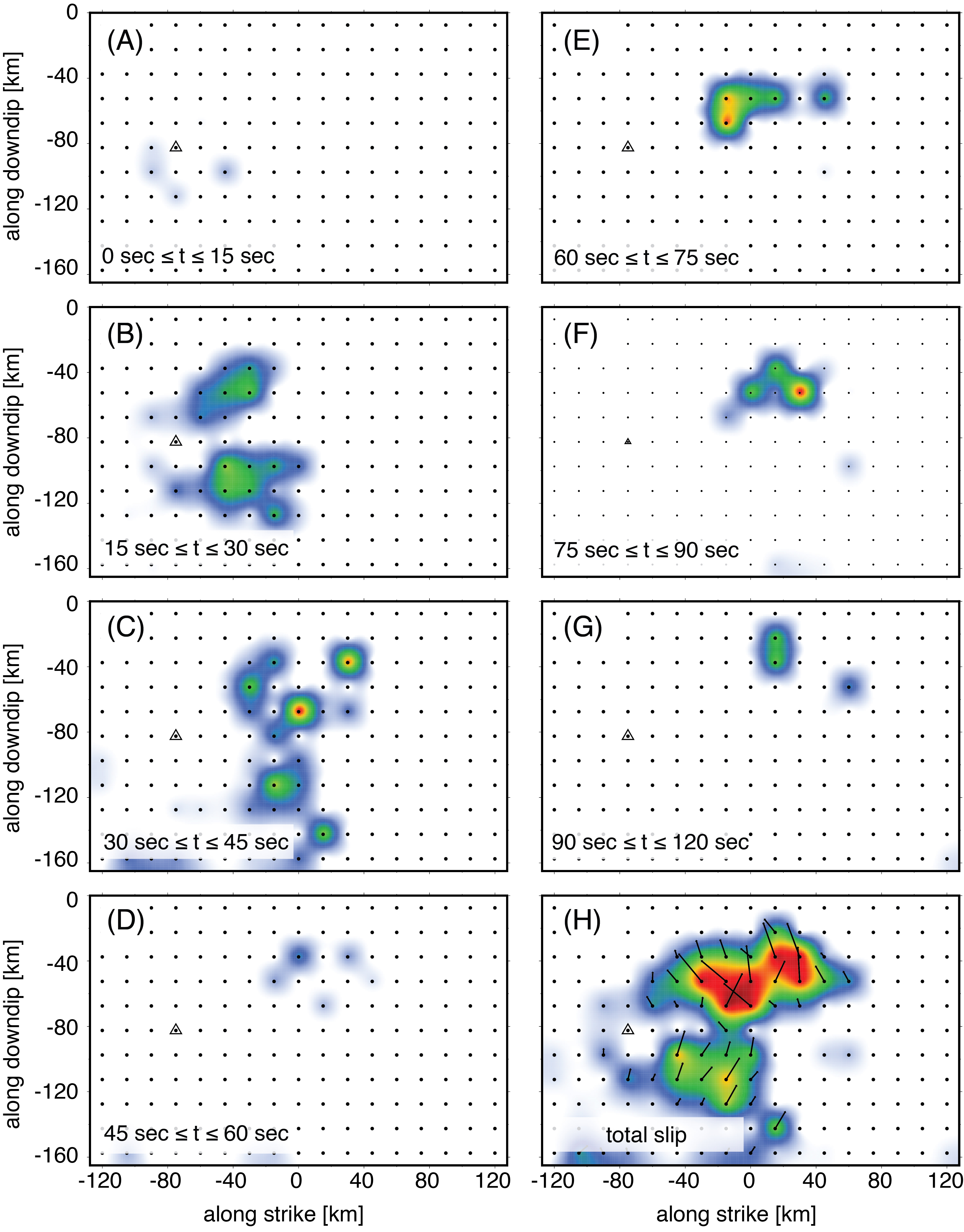
Figure S9. (a)–(f) Cumulative slip within 15 s intervals in the Gorkha slip model, determined from an inversion assigning equal weights to all available data. (g) Cumulative slip in our Gorkha slip model from 90 to 120 s. (h) Total cumulative slip in our joint Gorkha slip model. The color scale is as in Figure 2. The open black triangle is the Gorkha hypocenter, black dots are the centers of the subfaults in the Gorkha region, arrows indicate slip rake, red triangle is the Kodari hypocenter, red outline marks the location of the region of Kodari slip plotted at the right, and red dots are the subfault centers in the Kodari slip model.
European Space Agency InSARap program, http://insarap.org (last accessed May 2015).
Lindsey, E., R. Natsuaki, X. Xu, M. Shimada, H. Hashimoto, and D. Sandwell (2015). Line of sight deformation from ALOS-2 interferometry: Mw 7.8 Gorkha earthquake and Mw 7.3 aftershock, Geophys. Res. Lett. 42, doi: 10.1002/2015GL065385, also available at http://topex.ucsd.edu/nepal.
[ Back ]