This electronic supplement includes two figures showing seismograms before source normalization (Figs. S1 and S2) and two tables that compare estimates of crustal thickness from different back azimuths at stations FORT and WB2, respectively (Tables S1 and S2). The text below discusses in some detail how uncertainties in crustal thickness (H) and P wavespeed (VP) are determined.
Estimating Uncertainties of Crustal Thickness (H) and P Wavespeed (VP)
For a total number of n data points at each station, we express the linear equation (equation 2 of the main article) in matrix form
(S1)
in which d is the data vector cast in T2/4, G is the matrix containing corresponding values of p, and m is the model vector made of two unknowns, the interception and the slope being sought. That is,
(S2)
The well-known, generalized inverse solution to equation (S1) is then (Aster et al., 2005)
(S3)
The associated covariance matrix of m is also well established:
(S4)
in which cov(d) is the covariance matrix of d. In our case, cov(d) is a diagonal matrix, because measurements from different earthquake sources are independent.
(S5)
The variance of each element of d is derived from the variance of T, according to the rule for variance propagation as follows (e.g., Ku, 1966):
(S6)
Once m is estimated, it is trivial to find H and VP:
(S7)
in which a and b are the slope and the intercept in equation (2) of the main article, respectively, or
(S8)
Using rules for variance propagation (e.g., Ku, 1966), uncertainties of H and VP are calculated from those of a and b as
(S9)
in which σ2(a), σ2(b), and cov(a, b) are the variance of a, that of b, and the covariance between a and b, respectively. In other words, they are elements of cov(m):
(S10)
In Figures 2b, 5b, and 7b of the main article, the error bars are calculated by equation (S9). In each of these plots, to determine the region enclosing estimated values of H and VP at a confidence level of 68% or above, we first calculate the region in terms of parameters b and a and then projected the result into coordinates [H, VP] through equation (S7). This procedure is nonlinear, resulting in a distorted ellipse in the final plot.
Table S1. Estimates of crustal thickness using earthquakes from additional back azimuths at station FORT.
Table S2. Estimates of crustal thickness using earthquakes from additional back azimuths at station WB2.
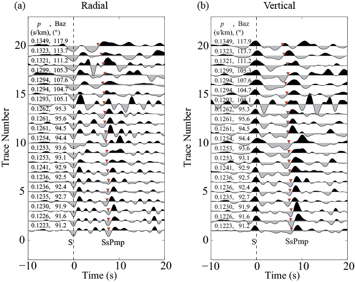
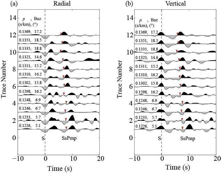
Figure S1. Examples of data from seismic station FORT. (a) Radial- and (b) vertical-component seismograms within a narrow back azimuth of 105°±15°; p is the ray parameter of the incoming S wave, and Baz is the back azimuth of each event. Red triangles mark the onset of the SsPmp phase. The seismograms are aligned by arrivals of the direct S phase on the radial component.
Figure S2. Data from station WB2. The layout is the same as that in Figure S1.
Aster, R. C., B. Borchers, and C. H. Thurber (2005). Parameter Estimation and Inverse Problems, Elsevier Academic Press, Burlington, Massachusetts.
Ku, H. H. (1966). Notes on the propagation of error formulas, J. Res. Natl. Bur. Stand. (U.S.) 70C, 263–273.
[ Back ]