This electronic supplement contains figures comparing observed and synthetic waveforms and Global Positioning System (GPS) displacements and spatial–temporal resolution and parameter tests, a movie showing wave propagation, and includes additional information about the data fittings of the inversion result and two inversion tests.
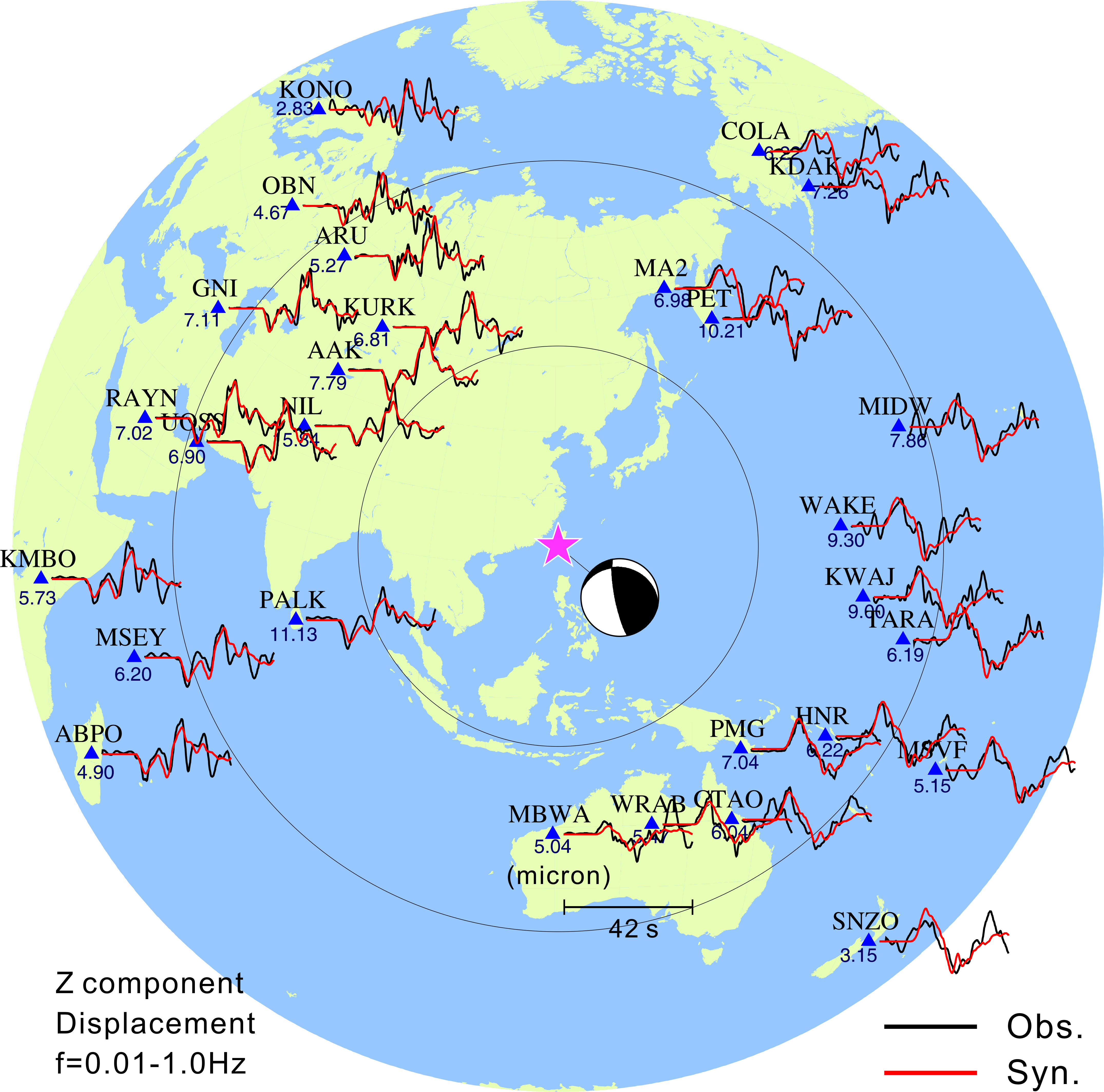
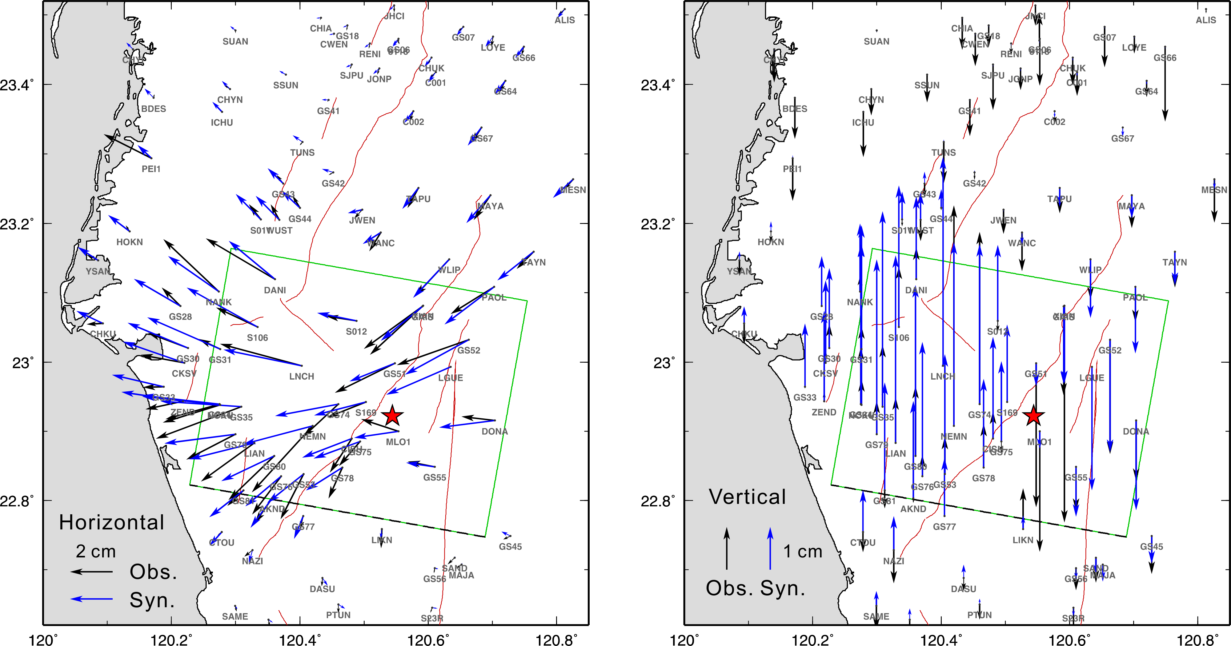
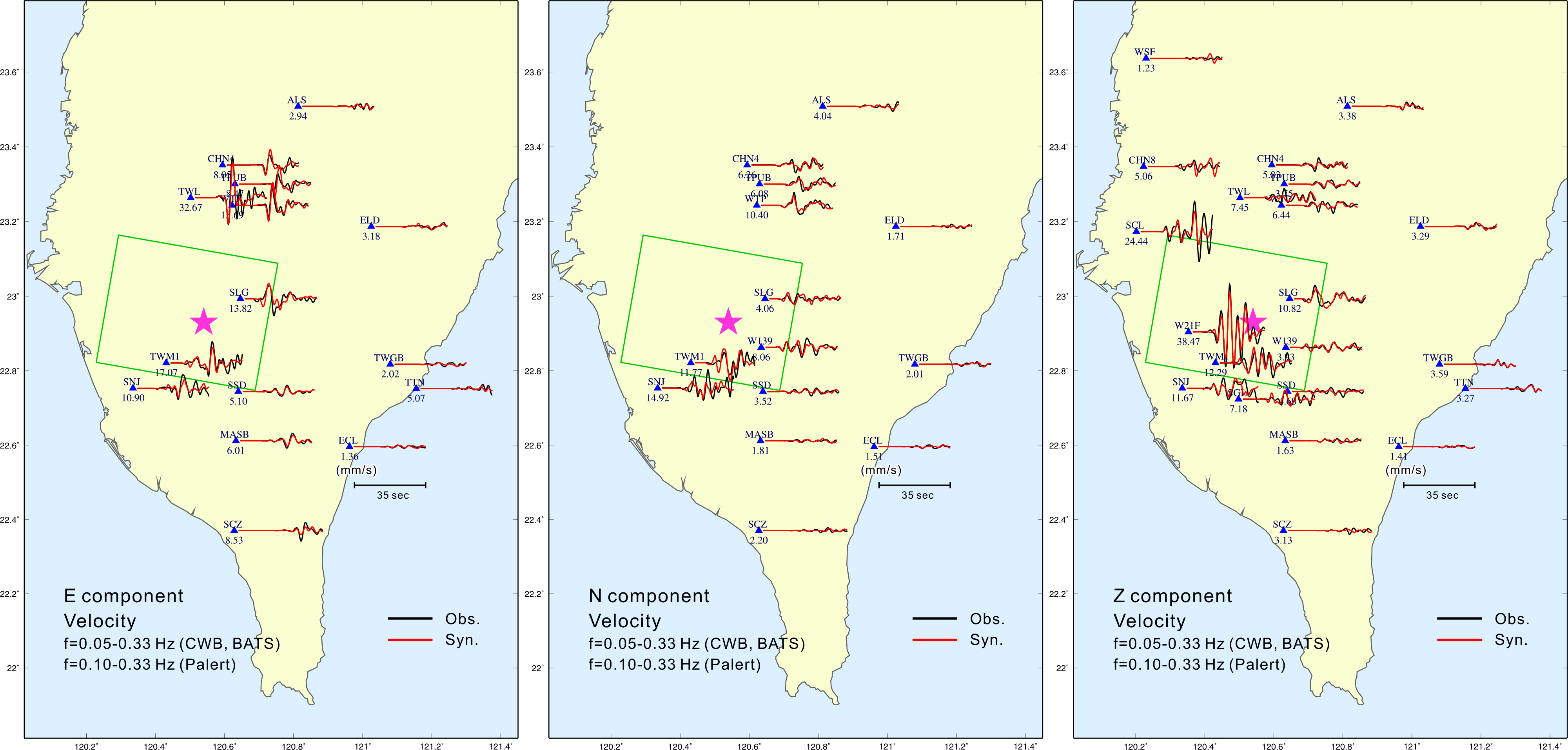
The synthetic and the observed teleseismic waveforms are displayed in Figure S1. The stations located to the west had larger discrepancies in waveforms, especially the later phases. In contrast, the stations located to the east show simpler waveforms, and their main characteristics were well fitted. The misfit of teleseismic data was 0.31. Figure S2 shows the comparison of synthetic and observed GPS coseismic displacements. The synthetics in horizontal component were comparable with observations. However, the vertical component did not fit well. The poor fitting is possibly due to data uncertainty. The secondary movements that occurred with the coseismic deformation could also influence the fitting. The GPS data misfit was 0.57. Comparison between local ground-motion waveforms and synthetic seismograms is provided in Figure S3. The fittings are acceptable not only for stations near the source area but also for distant stations. The waveform misfit of local ground-motion data was 0.31. The total misfit of the three data sets was 0.34.
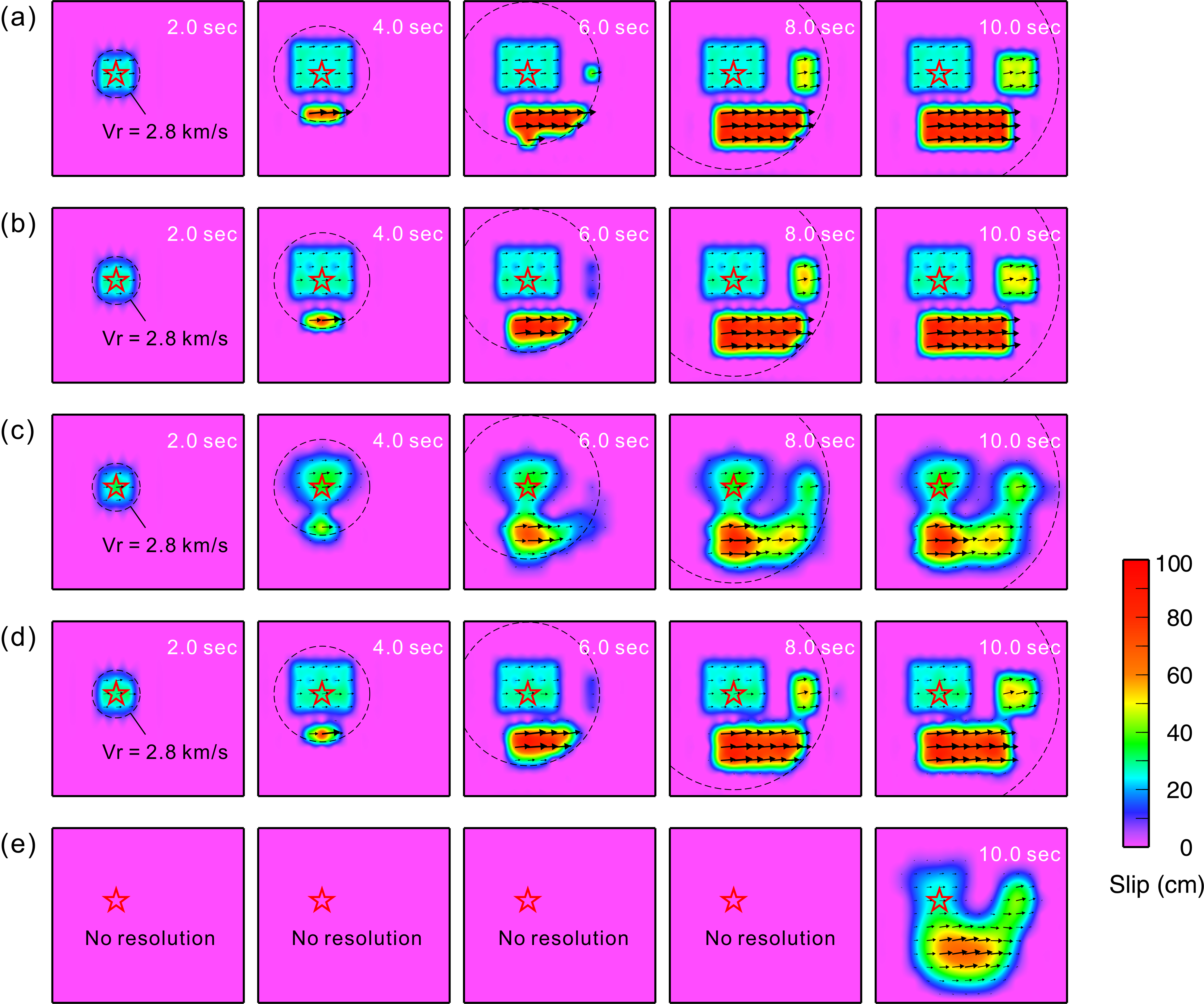
To appraise the spatial–temporal resolution of the inversion, a resolution test was performed. We generated the synthetic teleseismic, GPS, and local strong-motion data for the input test model using the same methods in Green’s function calculations. Then, inversions with different data sets were performed. Figure S4 shows the original input model and the inversion results derived with different settings: (a) input characteristic slip pattern, (b) joint inversion, (c) teleseismic only, (d) local ground motion only, and (e) GPS only. The rupture velocity (Vr) was set to 2.6 km/s in the input model (a). In (b), (c), and (d), the maximum Vr was set to 3.5 km/s. We used 30 time windows in the inversion and each have 0.4 s in length and offset by 0.2 s. A slip recovery rate, defined as [1 − (Σ|Slip of input − Slip of inverted|/Σ|Slip of input|)] × 100%, was used to evaluate the goodness of the result. A 100% recovery rate indicates the input rupture model (a) is totally recovered. The slip recovery rates determined from (b), (c), (d), and (e) are 91.6, 41.4, 64.9, and 38.2, respectively. This spatial–temporal resolution test shows the ability to resolve the rupture time history using joint source inversion. It is noted that the recovery rates were poor when using only one data set in the inversion. In addition, there is no temporal resolution when using GPS data alone.
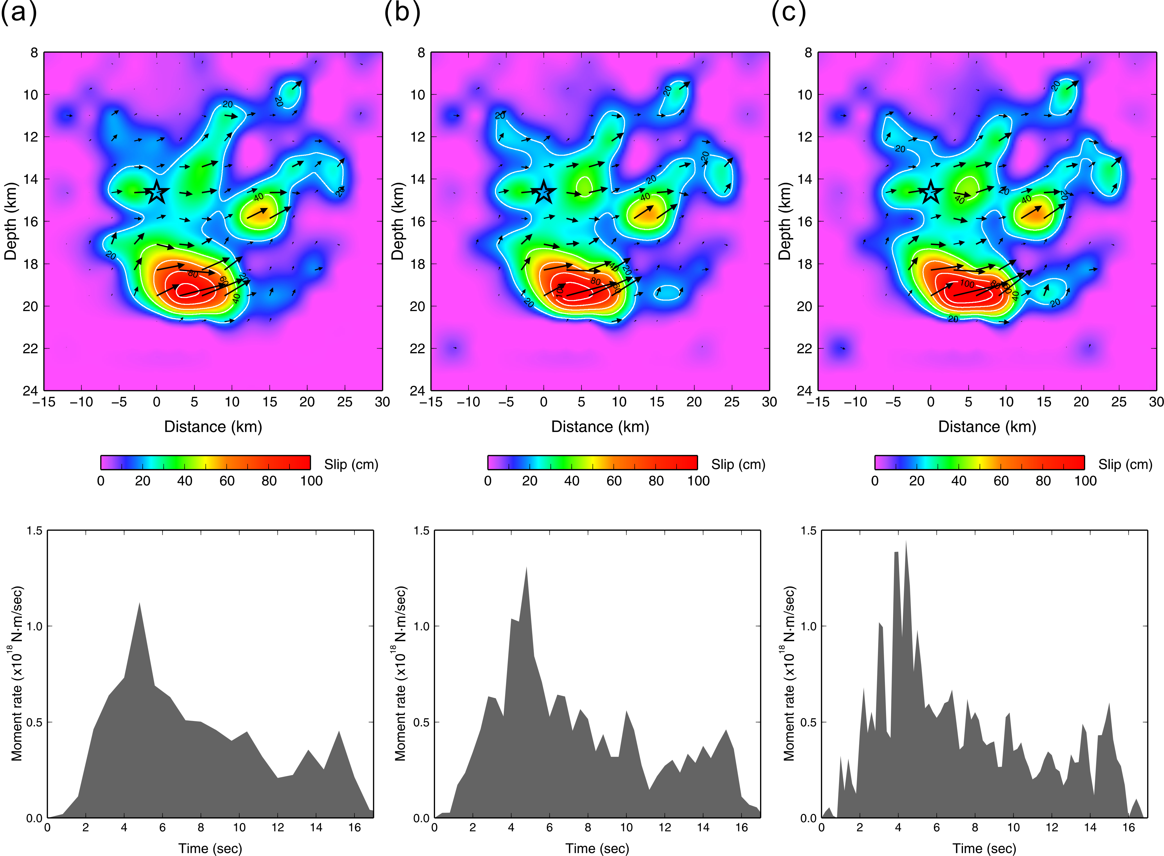
To examine the necessity of extra time window, we conducted a test using a different number of time windows. The same data set used for the joint inversion of the Meinong earthquake was considered in this test. Figure S5 shows the inversion results that adopt a different number of time windows: (a) 15 time windows (with 1.6 s in length and overlapping for 0.8 s); (b) 30 time windows (with 0.8 s in length and overlapping for 0.4 s); and (c) 60 time windows (with 0.4 s in length and overlapping for 0.2 s). These settings allow each subfault to slip within ∼12 s, represented by different temporal resolutions. The results show that slip patterns in all three cases are consistent. The data misfits of the three cases are 0.35, 0.34, and 0.33, respectively. The shapes of moment rate function are similar, in the way that they both have a large peak between ∼4–6 s and a total duration of ∼16 s. This test suggests that the inversion scheme is stable even in cases where large numbers of time windows are used. It is worth mentioning that the shorter time window not only improves temporal resolution in the whole rupture process but also provides more details of localized slip-rate function on each subfault. To demonstrate as many details as possible, the inversion result with 60 time windows with 0.4 s in length and overlapping for 0.2 s was discussed in this study.
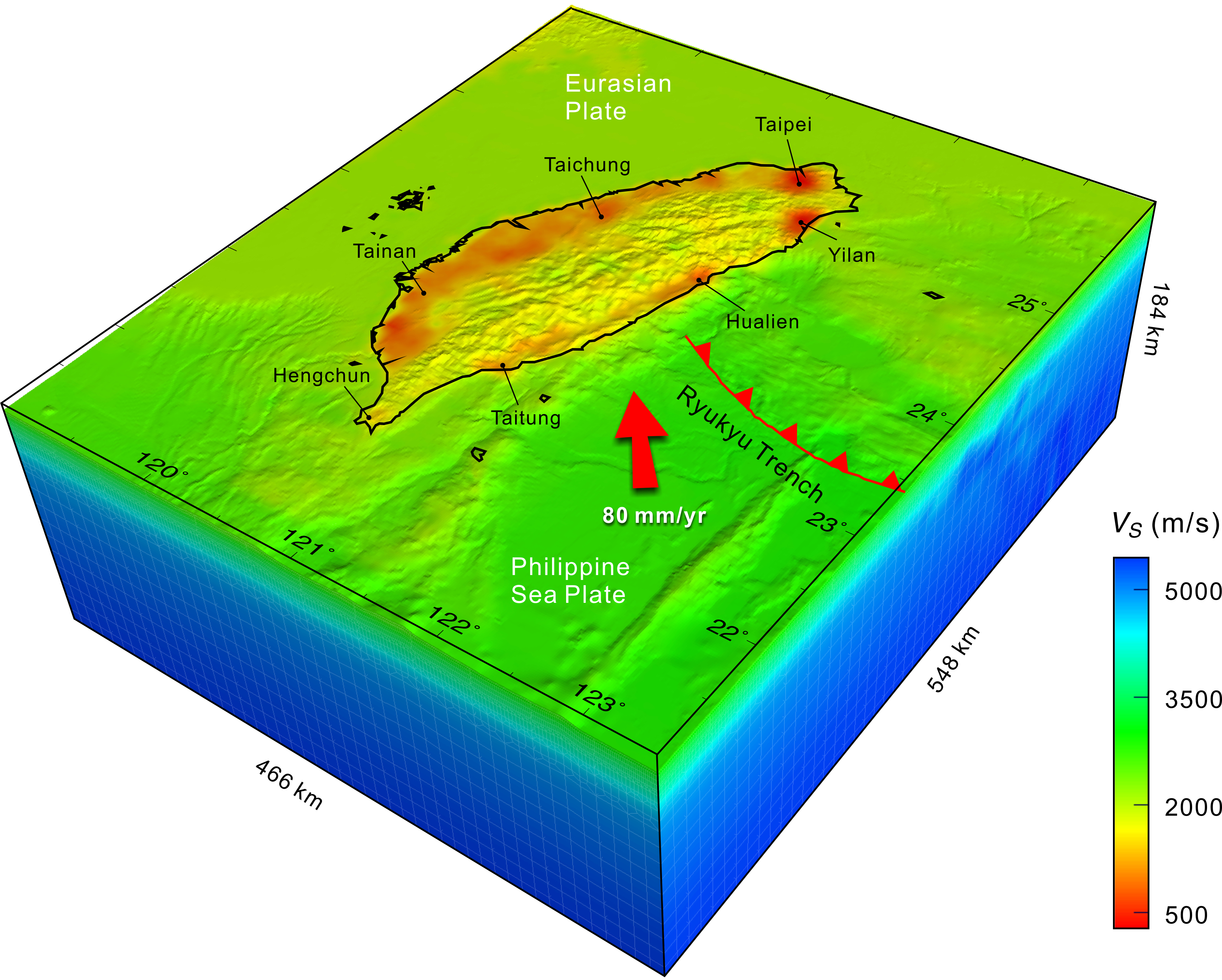
The spectral-element method (SEM) mesh model employed in this study is shown in Figure S6. The size of the mesh model is 466.01 km × 548.39 km horizontally and +3.93 km to −180.00 km vertically. Most of the currently available seismological and geological information have been incorporated in the model, including large-scale 3D velocity model, shallow sedimentary, and surface topography. The surface topography based on 40-m digital elevation model data is implemented at the top of the SEM mesh model. The 3D regional tomographic model was derived by Huang et al. (2014), which integrates the data of P- and S-wave travel times, S–P times, and the borehole logging data (VS30 [Kuo et al., 2012] for near-surface correction) into one system. The slowest shear-wave velocity in the mesh model is 443 m/s. The distances between Gauss–Lobatto–Legendre (GLL) points in the horizontal direction at the surface is 303.4 m. Considering the resolutions of the numerical mesh and the velocity model used, the simulation is capable of representing a 3D wavefield and synthetic waveforms that are accurate to 0.625 Hz. In this study, we used the period of 3–20 s for the local ground-motion simulation. There are ∼5 points per wavelength in the simulation. The simulations were carried out on Green cluster in the Institute of Earth Sciences, Academia Sinica. It requires 288 CPU cores and takes ∼6.8 hr to complete a 120-s ground-motion simulation.
Figure S1. Comparisons between observed and synthetic teleseismic waveforms. Black and red lines are the observed and synthetic waveforms, respectively. The star shows the Central Weather Bureau (CWB) epicenter, and the focal mechanism plot indicates the focal mechanism determined by the Global Centroid Moment Tensor (CMT). All the waveforms are displacement-type and are band-pass filtered by 0.01–1.0 Hz. The maximum observed ground displacement is shown at each station.
Figure S2. Comparison between observation and synthetic for coseismic GPS displacements. Black and blue arrows are the observed and synthetic displacements, respectively. The red star and the green rectangle indicate the epicenter and the fault plane of the Meinong earthquake, respectively. The red lines show the surface traces of active faults.
Figure S3. Comparisons between observed and synthetic local waveforms. Black and red lines are the observed and synthetic waveforms, respectively. The pink star and the green rectangle indicate the epicenter and the fault plane of the Meinong earthquake. All the waveforms are velocity-type. The CWB 24-bit and Broadband Array in Taiwan for Seismology (BATS; TPUB, MASB, and TWGB) records were band-pass filtered by 0.05–0.33 Hz. The Palert data (W21F and W139) were filtered by 0.1–0.33 Hz. The maximum observed ground velocity is shown at each station.
Figure S4. Spatial–temporal resolution test. (a) Input characteristic slip pattern, (b) joint inversion, (c) teleseismic only, (d) local ground motion only, and (e) GPS only. A reference rupture front with Vr = 2.8 km/s is shown by dashed circle.
Figure S5. Time-window number test. (a) 15 time windows (with 1.6 s in length and overlapping for 0.8 s); (b) 30 time windows (with 0.8 s in length and overlapping for 0.4 s); and (c) 60 time windows (with 0.4 s in length and overlapping for 0.2 s). The upper panels show the slip distributions, and lower panels are the moment rate functions determined from the three cases.
Figure S6. Spectral-element mesh model. The size of the region is 466.01 km × 548.39 km horizontally and +3.93 km to −180.00 km vertically. Most of the currently available relevant seismological and geological information have been incorporated in the model, including surface topography, shallow sedimentary (VS30; Kuo et al., 2012), and large-scale 3D wavespeed heterogeneity information (Huang et al., 2014). Background colors show the VS velocity, the slowest VS in the mesh is 443 m/s.
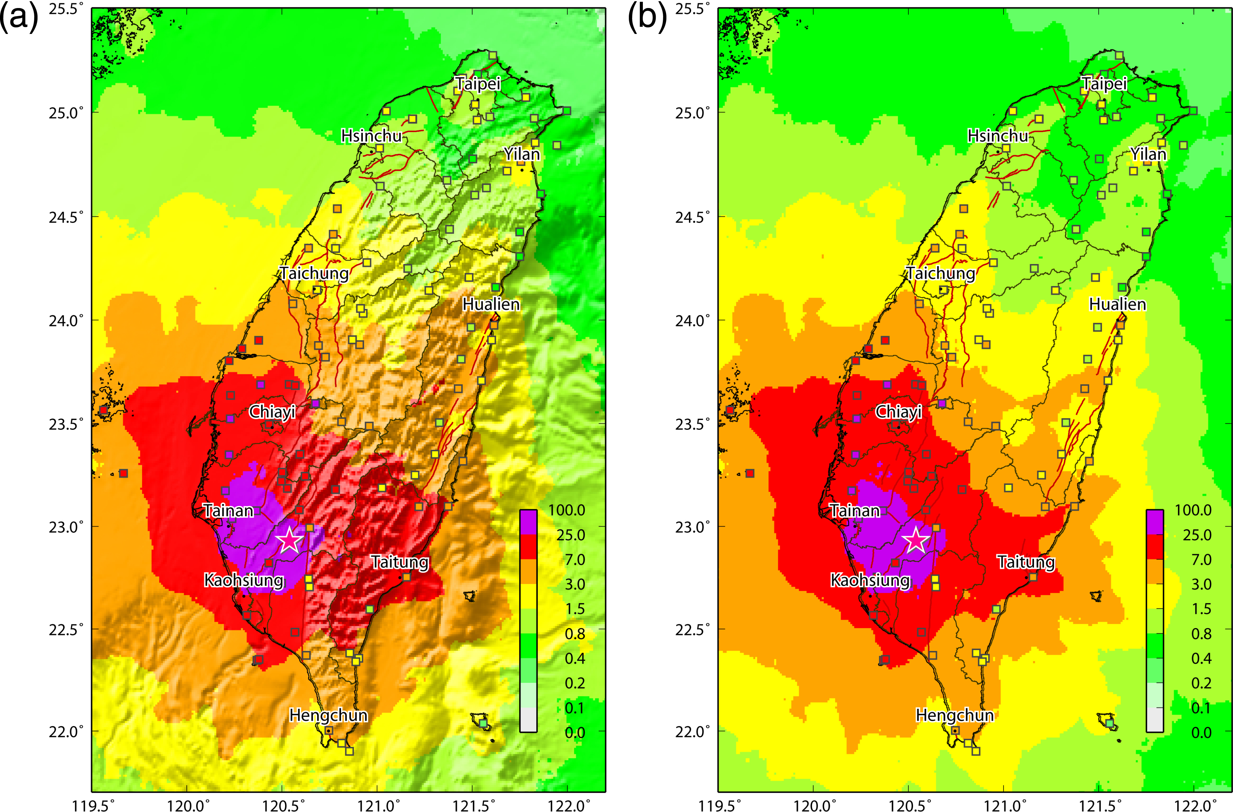
Figure S7. Comparison between simulations with and without topography. (a) 3D velocity with surface topography. (b) 3D velocity with flat surface at top of the model.
Download/View: Movie S1 [h.264-Encoded MP4 movie; ~26 MB]. Animation of 3D wave propagation simulation of the 2016 Meinong earthquake. The east–west component velocity wavefield is displayed.
Huang, H. H., Y. M. Wu, X. Song, C. H. Chang, S. J. Lee, T. M. Chang, and H. H. Hsieh (2014). Joint VP and VS tomography of Taiwan: Implications for subduction-collision orogeny, Earth Planet. Sci. Lett. 392, 177–191.
Kuo, C. H., K. L. Wen, H. H. Hsieh, C. M. Lin, T. M. Chang, and K. W. Kuo (2012). Site classification and VS30 estimation of free-field TSMIP stations using the logging data of EGDT, Eng. Geol. 129/130, 68–75.
[ Back ]