This electronic supplement contains tables of ocean-bottom seismometer (OBS) locations with recording start and end times, list of earthquakes on land used to identify the detection limits of OBSs, and station information, figures of probability density functions (PDFs) and waveforms, and tar file of waveform data.
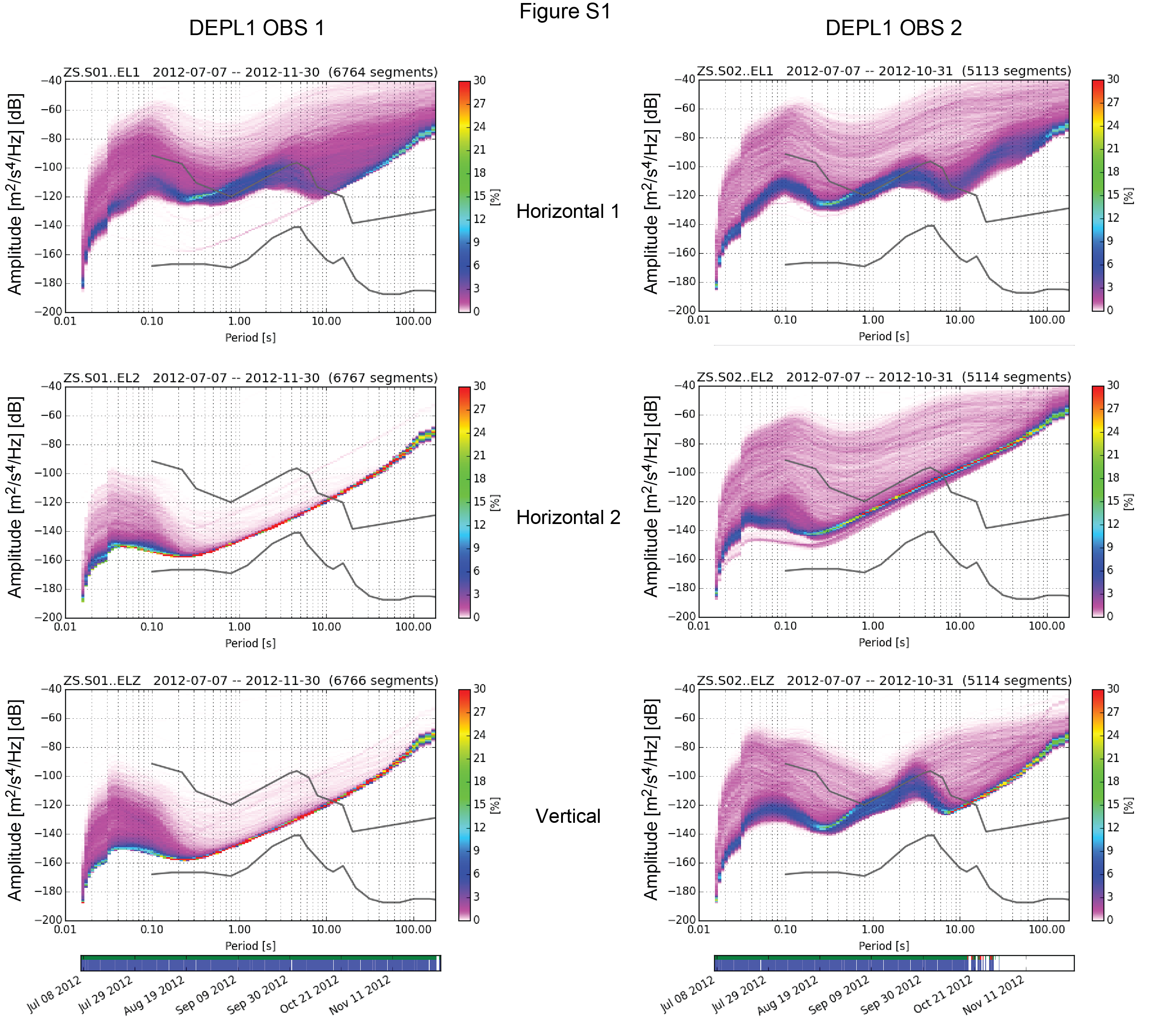
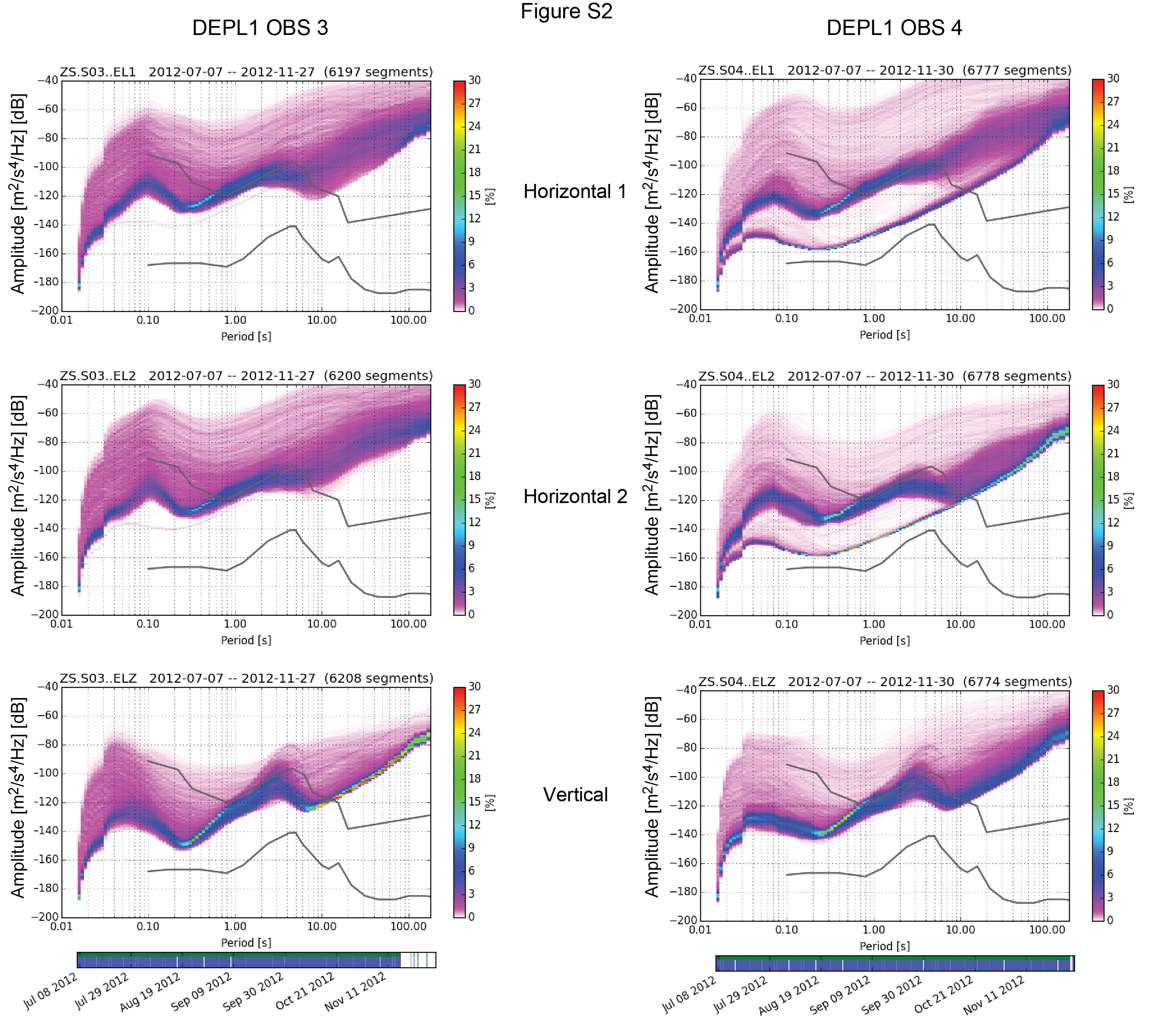
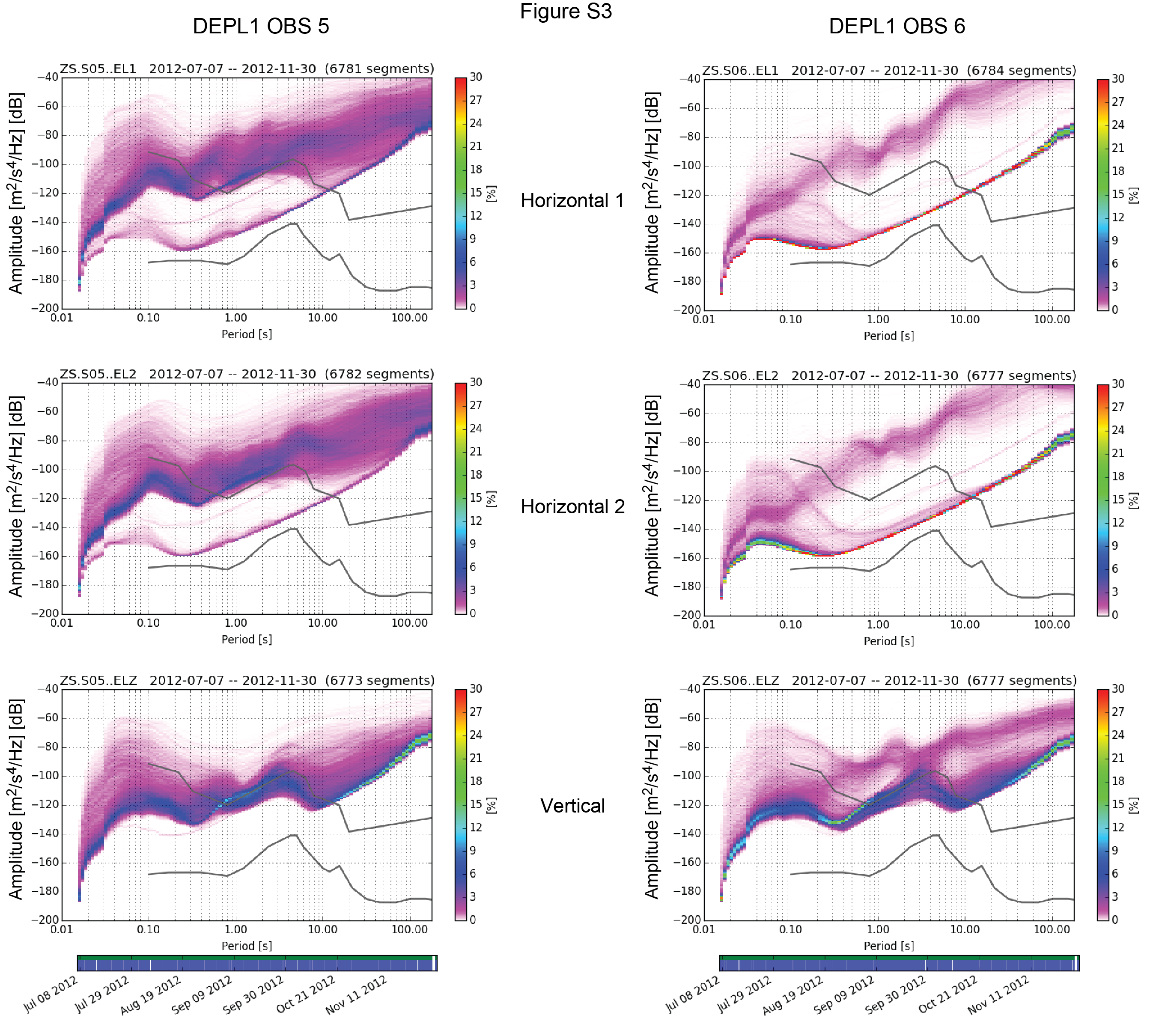
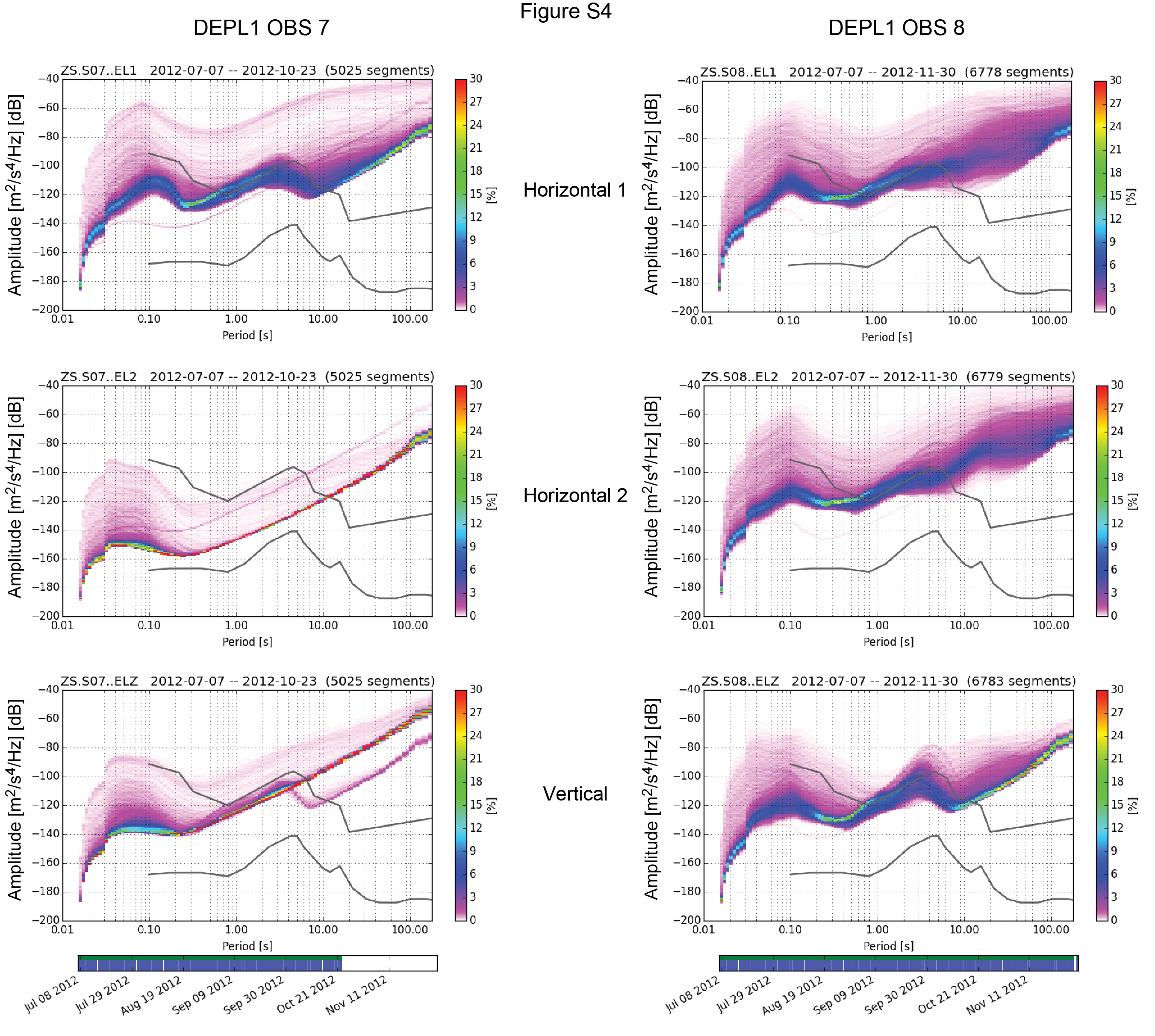
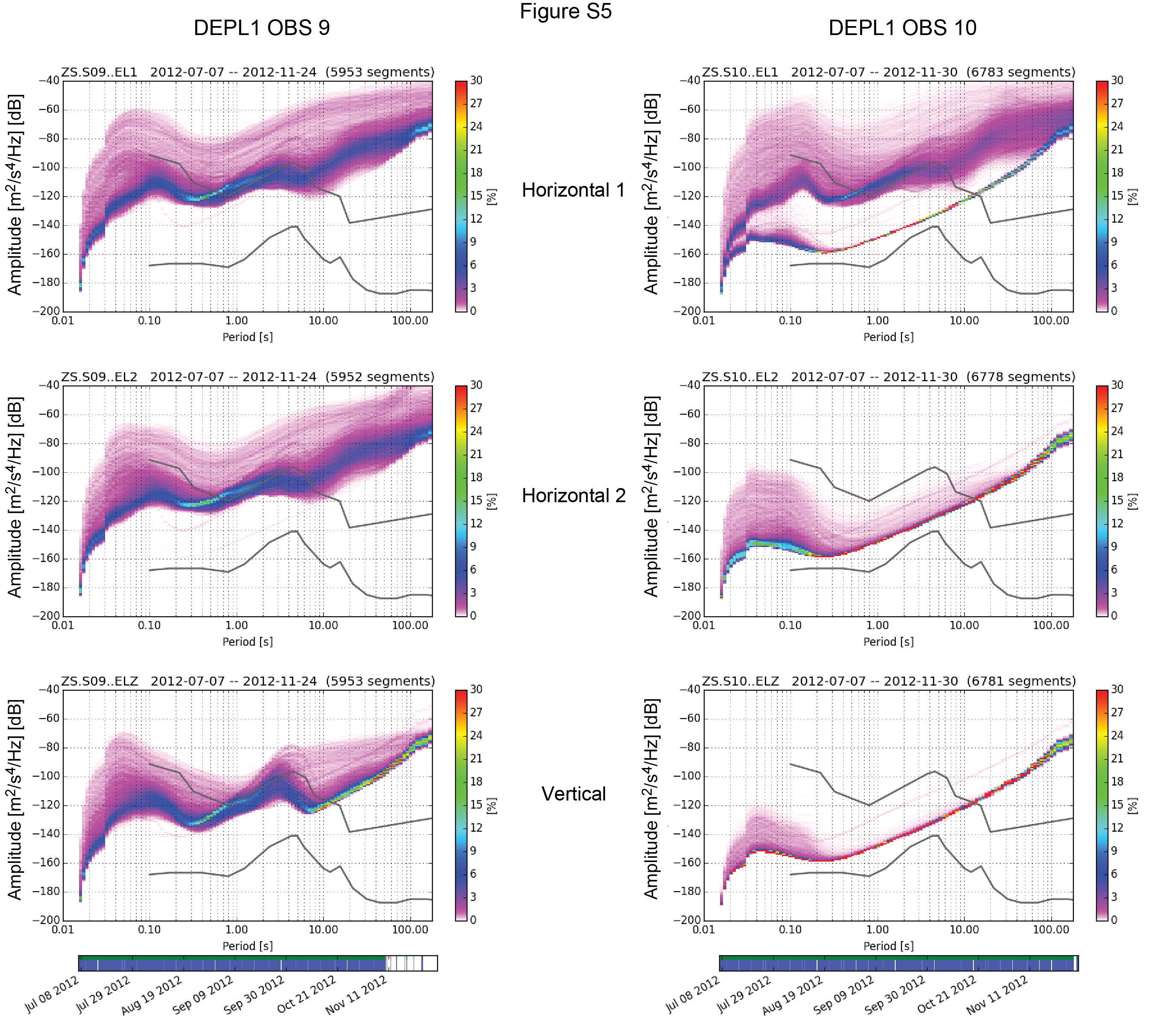
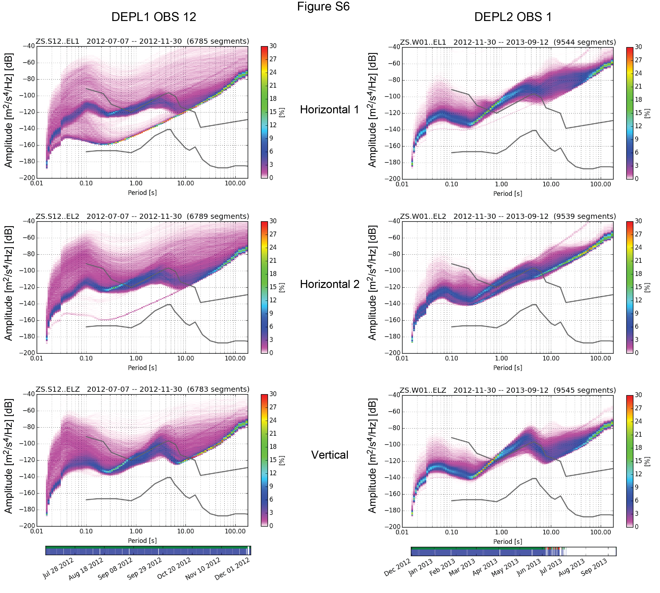
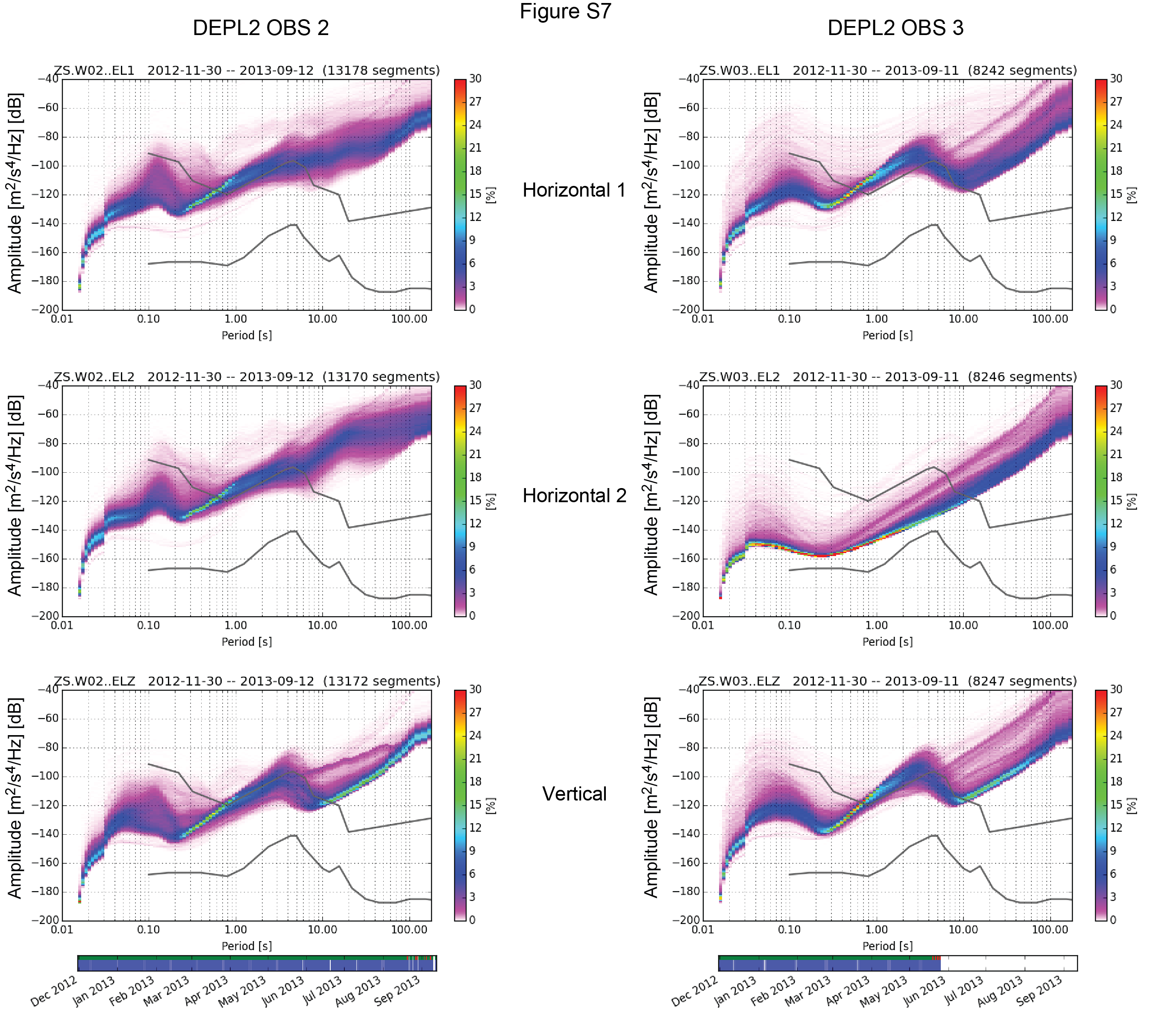
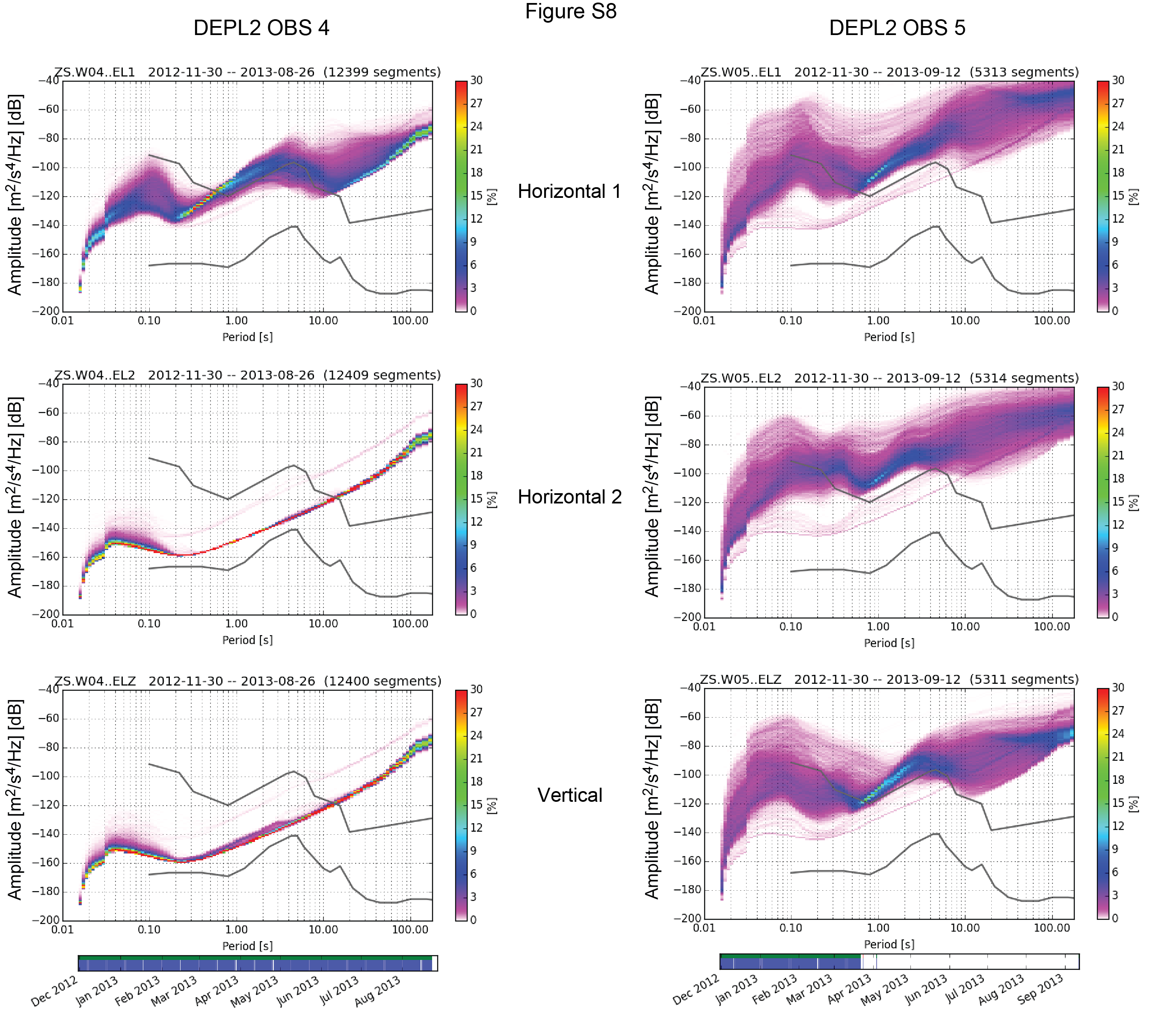
For all OBSs, Figures S1–S8 show PDF plots of the power spectral density (PSD). Each column is labeled for the deployment and corresponding OBS number. Each column contains the two horizontal (EL1 and EL2) and vertical (ELZ) components. The location and depths of each OBS is shown in Figure 2 of the main article and Table S1. The bottom bar shows the time range of each OBS. The top row shows data fed into the PSD; green patches represent available data; and red patches represent gaps in streams that were added to the probabilistic power spectral density (PPSD), the statistical analysis plot to show the amplitude occurrence of a given power at a particular period. The bottom row in blue shows the single PSD measurements that go into the histogram. The default processing method fills gaps with zeros, and these data segments then show up as single outlying PSD lines (Beyreuther et al., 2010). Specific data collection dates are given in Table S1. The color bar to the right indicates the probability that recorded data will fall within a certain power spectral level at a given frequency for the entire recording period of the OBS (the bar at the bottom). A time increment bin of 3600 s (1 hr) is used to calculate the PSD. The number of 1-hr segments used is noted on the top right corner labeled as segments. The solid gray lines show the high- and low-noise models from the measurement of Global Seismic Network (GSN) stations from Peterson (1993). The warmest colors on the plots represent the median noise level of the station component. The PDF helps determine the overall station data quality and the noise level at a station. Using the McNamara and Buland (2004) descriptions of seismic noise sources, we can look at the OBS PDF plots to identify where stations were not well coupled to the ground, when there is little variability in amplitudes beyond the background on some of its components.
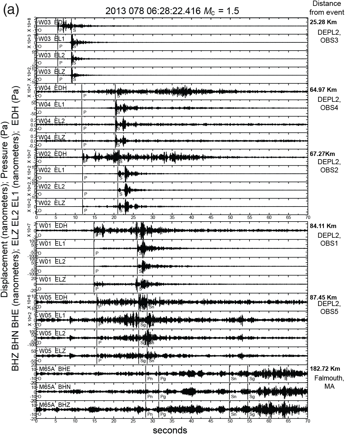
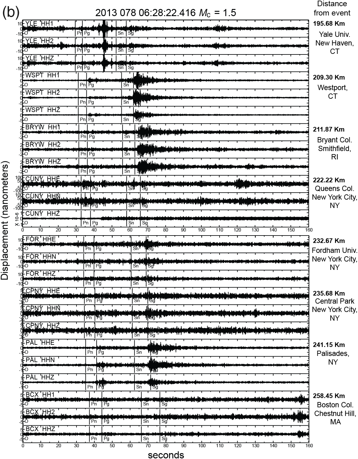
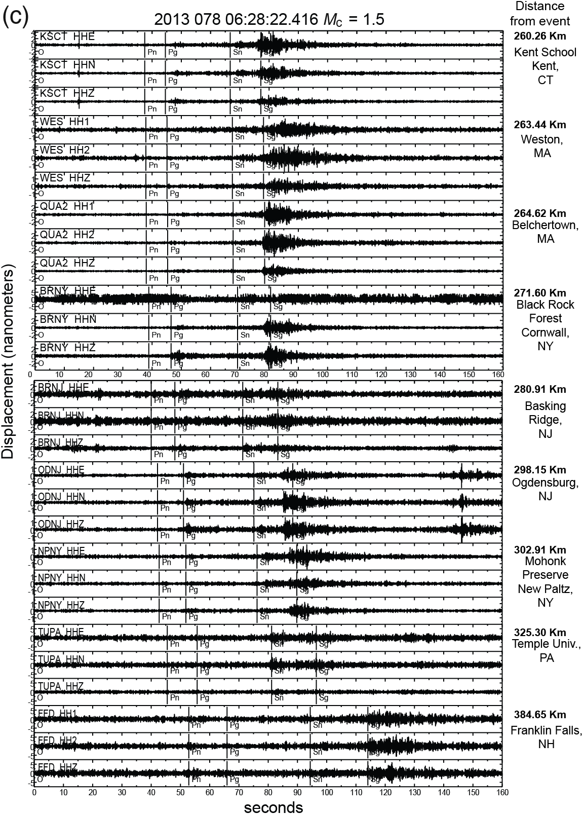
Waveform plots of the detected earthquake event of 19 March 2013 (Julian Date [JD] 078) 06:28:22.416 Mc 1.5. The seismograms have all been instrument corrected to show displacement in nanometers or pressure in pascals in the case of the hydrophone. They were filtered using a Butterworth-bandpass with corner frequencies at 5–15 Hz. The X axis is time in seconds from earthquake origin time. The Y axis is either pressure in pascals for hydrophones or displacement in nanometers for both broadband (BH) and high broadband (HH). Seismograms are plotted in order of distance from the earthquake with distance in kilometers shown on the right. Picked P and S arrivals are shown for the DEPL2 OBS. All other arrivals shown (Pn, Pg, Sn, and Sg) are predicted arrivals using IASP-91 velocity model (Kennett and Engdahl, 1991). The location name for each station is also labeled on the right below distance from event.
Table S1. Location of OBSs and their recording start and end dates.
Table S2 [Plain Text Comm-separated values; 16 KB]. List of earthquakes on land used to identify the detection limits of the OBSs during DEPL1. The list includes suspected or verified blasts from local mining or quarry activities and is primarily of magnitude Mc < 2.0. DEPL1 OBS 3 was used to calculate the approximate event–OBS distances in kilometers.
Table S3. Maine MLg 4.5, 16 October 2012 (JD 290) 23:12:22.0 UTC (−70.68, 43.59) depth = 6.6 km, earthquake. Information of stations used for the study of the event including event to station distance and azimuth. Stations ending in .LD are from the Lamont–Doherty Cooperative Seismographic Network (LCSN).
Table S4. Rockport Mc 2.7, 16 September 2012 (JD 260) 02:31:37.6 UTC (−69.84, 42.70) depth = 1.72 km, earthquake. Information of the stations used to study the event including event to station distance and azimuth. Stations ending in .LD are from the LCSN. Stations ending in .NE are from the New England Seismic Network (NESN).
Table S5 [Plain Text Comm-separated values; 25 KB]. List of earthquakes during DEPL2 with the same search area as DEPL1. The list includes suspected or verified blasts from local mining or quarry activities and is primarily of magnitude Mc <2.0. All DEPL2 OBSs are used to calculate the approximate event–OBS distances in kilometers.
Figure S1. PDF plot for DEPL1 OBS 1 and DEPL1 OBS 2.
Figure S2. PDF plot for DEPL1 OBS 3 and DEPL1 OBS 4.
Figure S3. PDF plot for DEPL1 OBS 5 and DEPL1 OBS 6.
Figure S4. PDF plot for DEPL1 OBS 7 and DEPL1 OBS 8.
Figure S5. PDF plot for DEPL1 OBS 9 and DEPL1 OBS 10.
Figure S6. PDF plot for DEPL1 OBS 12 and DEPL2 OBS 1.
Figure S7. PDF plot for DEPL2 OBS 2 and DEPL2 OBS 3.
Figure S8. PDF plot for DEPL2 OBS 4 and DEPL2 OBS 5.
Figure S9. (a) For the DEPL2 OBS, the hydrophone (EDH), horizontals (EL1 and EL2), and vertical (ELZ) components are plotted in that order. The hydrophone is in pressure units of pascals, whereas the seismometers are in units of nanometers. For the TA-M65A broadband, Falmouth, Massachusetts, horizontals (BHE and BHN) and vertical (BHZ) are plotted. (b and c) Land station high broadband are plotted, horizontals first (HH1 and HH2 or HHE and HHN), then vertical (HHZ).
The compressed file SA-timeHistoryData.zip contains ASCII version of the acceleration waveform used to calculate the spectral acceleration. These files end in .sg2. The calculated spectral accelerations from each of these waveforms are included in the compressed file as text files. The README.txt file describes the contents of both types of files. The two events are in separate folders, Maine-2012/ and Rockport-2012/. Pre-event waveforms have also been included in their respective folders for each earthquake.
Download: SA-timeHistoryData.zip [Zip Archive; ~10.6 MB].
Beyreuther, M., R. Barsch, L. Krischer, T. Megies, Y. Behr, and J. Wassermann (2010). ObsPy: A Python toolbox for seismology, Seismol. Res. Lett. 81, no. 3, 530–533, doi: 10.1785/gssrl.81.3.530.
Kennett, B. L. N., and E. R. Engdahl (1991). Traveltimes for global earthquake location and phase identification, Geophys. J. Int. 105, no. 2, 429–465, doi: 10.1111/j.1365-246X.1991.tb06724.x.
McNamara, D. E., and R. P. Buland (2004). Ambient noise levels in the continental United States, Bull. Seismol. Soc. Am. 94, no. 4, 1517–1527, doi: 10.1785/012003001.
Peterson, J. R. (1993). Observation and modeling of seismic background noise, U.S. Geol. Surv. Open-File Rept. 93-322, 94 pp.
[ Back ]