This electronic supplement contains MATLAB MITP_USA_2016MAY model and plotting scripts, figures of checkerboard tests, and animations of model evolution.
MIT P-wave tomography model for the United States, MITP_USA_2016MAY, created using travel-time residuals from the global Engdahl–van der Hilst–Buland (EHB) catalog plus USArray Transportable Array from 2004 to May 2016.
The model is provided as a .mat file comprised of velocity perturbations relative to ak135 at node points. To allow for better investigation of the model, we present the model on the original irregular grid used for inversion and include scripts for reading and interpreting it. The .mat file contains an array with rows representing each mantle volume in the irregular grid and columns representing the following:
This update also includes a MATLAB library for plotting cross sections and map sections from the new model. Scripts were tested in MATLAB v.8.1.0. Example outputs are shown in Figures S1 and S2.
Animation combining a moving camera position and slicing to illustrate the 3D geometry of the MITP_USA_2016MAY+scirpts. Geographic reference is provided by coast and political boundaries drawn in an orange color. Yellow and white flow lines illustrate the direction of Farallon-North America plate motion and the Cape Mendocino slab window (Pavlis et al., 2012) and the southern connection of the Farallon slab to the subduction zones in Central America (Panessa, 2013). The yellow flow lines drawn from the active trench in Mexico and the white lines are northward projections estimated by a reconstruction of the opening of the Gulf of California and related southward step in the subduction zone. At 12 s, the scene is rotated to a view over Mexico, and slices through the model appear. Magenta surfaces show 410 and 660 km discontinuity from Wang and Pavlis (2016). The remainder of the animation slices the tomography model on a plane approximately parallel to the average Farallon-North America plate motion beginning with the slicing plane crossing the southeastern United States and ending where the plane crosses the northwest corner of the contiguous United States in the state of Washington. At 24 s, the flow lines from Central America disappear, and the edge defined by the Mendocino slab window is drawn as a black surface. That surface, along with the 410 and 660 km discontinuities, is clipped 50 km in front of the slice to provide a perspective.
To visualize the effects that USArray has on the recovery of mantle structure, we create a series of models through time. From the inception of the array to May 2016, we add cumulative USArray data in one-month increments to the inversion on the final adaptive grid. The resulting models viewed in order show the dramatic improvement in illumination through time and provide a better sense of the effects of specific parts of the array. Animations include maps, cross sections across the contiguous United States, and checkerboard resolution tests.
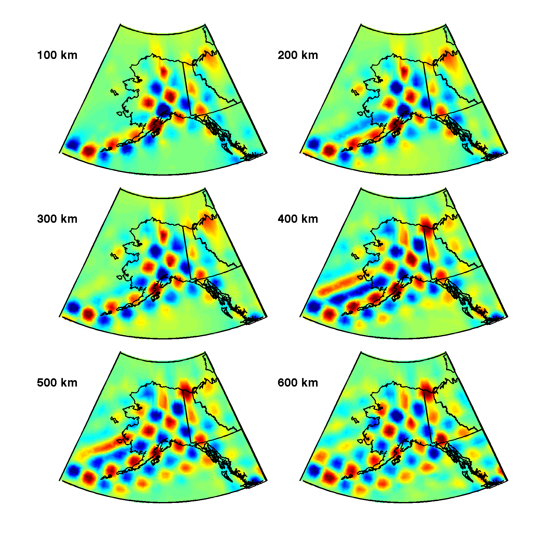
Two sets of checkerboard resolution tests were performed to assess the recovery of seismic structure. The input model for the first resolution test (Fig. S3) was a checkerboard with 1.5° × 1.5° beneath the contiguous United States. For the second test (Fig. S4), a model with 3° × 3° pattern was rotated so that checks of 3° were positioned beneath Alaska.
Resolution tests were used to quantify the recovery of heterogeneity using the resolving power metric (Burdick et al., 2014). The input model and recovered model are compared to each other with a weighting function chosen to have the same spatial wavelength of the input checkers. Nonshaded regions in Figures 2–5 of the main article show where resolving power exceeds a threshold value of 0.65.
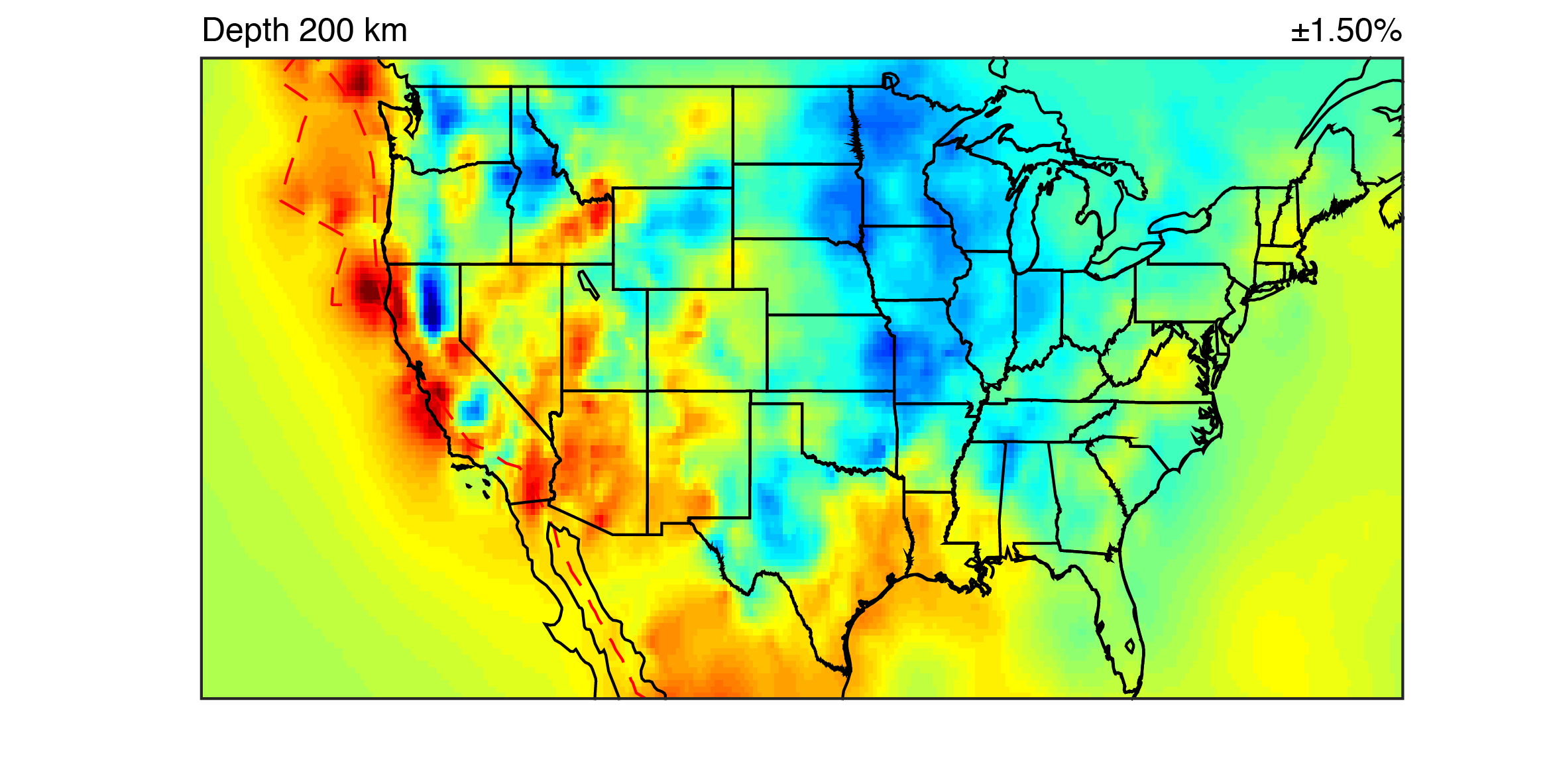
Figure S1. Example map section at 200 km depth from MITP_USA_2016MAY plotted with included scripts.
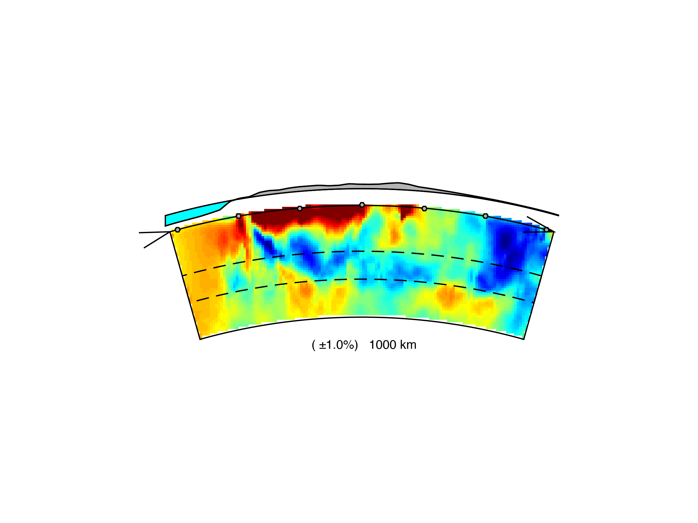
Figure S2. Example cross section plotted with included scripts.
Figure S3. Checkerboard resolution tests beneath contiguous United States. Checkers are 1.5° × 1.5° in scale.
Figure S4. Checkerboard resolution tests beneath Alaska, ±1.0 dV/V. Checkers are 3° × 3° in scale.
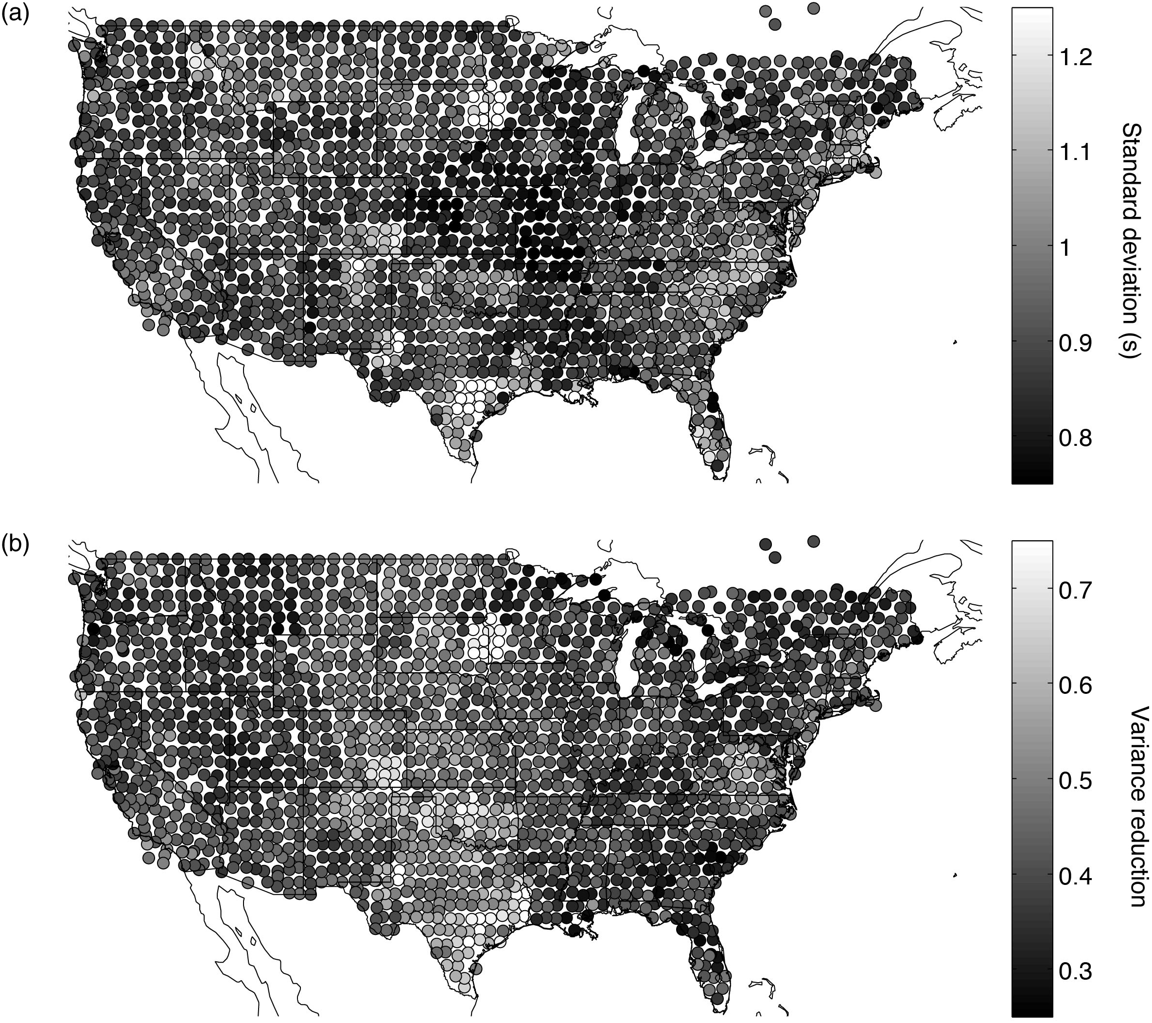
Figure S5. (a) Standard deviation in seconds of USArray travel-time residuals prior to inversion. The color of the marker at each station location represents the standard deviation of summary data to which that station contributed. (b) Reduction in variance of USArray residuals following the inversion. Marker color at each station location represents the reduction in the variance of summary data to which that station contributed, that is, the ratio of variance of residuals in MITP_USA_2016MAY to variance of residuals in ak135. The regional variation in the variance of the travel-time residuals and its reduction are affected not only by the heterogeneity beneath the array but also by far-field effects, including source distribution and near-source heterogeneity.
Download: 3DSliceWithTZsurface.mp4 [h.264-encoded MPEG4 movie; ~37.1 MB].
MITP_dep100_v2_movie.mp4 [h.264-encoded MPEG4 movie; ~7.3 MB].
MITP_dep200_v2_movie.mp4 [h.264-encoded MPEG4 movie; ~7.7 MB].
MITP_dep300_v2_movie.mp4 [h.264-encoded MPEG4 movie; ~7.9 MB].
MITP_dep400_v2_movie.mp4 [h.264-encoded MPEG4 movie; ~8.0 MB].
MITP_dep500_v2_movie.mp4 [h.264-encoded MPEG4 movie; ~7.9 MB].
MITP_dep600_v2_movie.mp4 [h.264-encoded MPEG4 movie; ~7.9 MB].
MITP_dep700_v2_movie.mp4 [h.264-encoded MPEG4 movie; ~7.9 MB].
MITP_dep800_v2_movie.mp4 [h.264-encoded MPEG4 movie; ~8.0 MB].
MITP_dep1300_v2_movie.mp4 [h.264-encoded MPEG4 movie; ~8.1 MB].
MITP_dep1600_v2_movie.mp4 [h.264-encoded MPEG4 movie; ~8.1 MB].
MITP_dep2000_v2_movie.mp4 [h.264-encoded MPEG4 movie; ~8.1 MB].
MITP_dep2500_v2_movie.mp4 [h.264-encoded MPEG4 movie; ~8.0 MB].
MITPslice_25N_movie.mp4 [h.264-encoded MPEG4 movie; ~3.2 MB].
MITPslice_26N_movie.mp4 [h.264-encoded MPEG4 movie; ~3.3 MB].
MITPslice_27N_movie.mp4 [h.264-encoded MPEG4 movie; ~3.4 MB].
MITPslice_28N_movie.mp4 [h.264-encoded MPEG4 movie; ~3.4 MB].
MITPslice_29N_movie.mp4 [h.264-encoded MPEG4 movie; ~3.3 MB].
MITPslice_30N_movie.mp4 [h.264-encoded MPEG4 movie; ~3.3 MB].
MITPslice_31N_movie.mp4 [h.264-encoded MPEG4 movie; ~3.3 MB].
MITPslice_32N_movie.mp4 [h.264-encoded MPEG4 movie; ~3.2 MB].
MITPslice_33N_movie.mp4 [h.264-encoded MPEG4 movie; ~3.2 MB].
MITPslice_34N_movie.mp4 [h.264-encoded MPEG4 movie; ~3.2 MB].
MITPslice_35N_movie.mp4 [h.264-encoded MPEG4 movie; ~4.8 MB].
MITPslice_36N_movie.mp4 [h.264-encoded MPEG4 movie; ~4.8 MB].
MITPslice_37N_movie.mp4 [h.264-encoded MPEG4 movie; ~4.9 MB].
MITPslice_38N_movie.mp4 [h.264-encoded MPEG4 movie; ~4.9 MB].
MITPslice_39N_movie.mp4 [h.264-encoded MPEG4 movie; ~4.8 MB].
MITPslice_40N_movie.mp4 [h.264-encoded MPEG4 movie; ~4.7 MB].
MITPslice_41N_movie.mp4 [h.264-encoded MPEG4 movie; ~4.5 MB].
MITPslice_42N_movie.mp4 [h.264-encoded MPEG4 movie; ~4.4 MB].
MITPslice_43N_movie.mp4 [h.264-encoded MPEG4 movie; ~4.3 MB].
MITPslice_44N_movie.mp4 [h.264-encoded MPEG4 movie; ~4.1 MB].
MITPslice_45N_movie.mp4 [h.264-encoded MPEG4 movie; ~3.9 MB].
MITPslice_46N_movie.mp4 [h.264-encoded MPEG4 movie; ~3.8 MB].
MITPslice_47N_movie.mp4 [h.264-encoded MPEG4 movie; ~3.7 MB].
MITPslice_48N_movie.mp4 [h.264-encoded MPEG4 movie; ~3.5 MB].
Res100_USonly_movie.mp4 [h.264-encoded MPEG4 movie; ~4.3 MB].
Res200_USonly_movie.mp4 [h.264-encoded MPEG4 movie; ~5.5 MB].
Res300_USonly_movie.mp4 [h.264-encoded MPEG4 movie; ~5.5 MB].
Res400_USonly_movie.mp4 [h.264-encoded MPEG4 movie; ~5.3 MB].
Res500_USonly_movie.mp4 [h.264-encoded MPEG4 movie; ~6.8 MB].
Res600_USonly_movie.mp4 [h.264-encoded MPEG4 movie; ~7.0 MB].
Download: MITP_USA_2016MAY+scripts.zip [Zipped archive of MATLAB file (.mat) and scripts (.m); ~8.1 MB].
Burdick, S., R. D. van der Hilst, F. L. Vernon, V. Martynov, T. Cox, J. Eakins, G. H. Karasu, J. Tylell, L. Astiz, and G. L. Pavlis (2014). Model update January 2013: Upper mantle heterogeneity beneath North America from travel-time tomography with global and USArray Transportable Array data, Seismol. Res. Lett. 85, no. 1, 77–81.
Panessa, A. (2013). Evidence for a coherent southeastern edge of the Farallon slab window from USArray tomography models, M.S. Thesis, Indiana University, Bloomington, Indiana.
Pavlis, G. L., K. Sigloch, S. Burdick, M. J. Fouch, and F. L. Vernon (2012). Unraveling the geometry of the Farallon plate: Synthesis of three-dimensional imaging results from USArray, Tectonophysics 532, 82–102.
Wang, Y., and G. L. Pavlis (2016). Roughness of the mantle transition zone discontinuities revealed by high-resolution wavefield imaging, J. Geophys. Res. 121, doi: 10.1002/2016JB013205.
[ Back ]