This electronic supplement contains recorded and synthetic interferograms, figures of trade-off between fault parameters, checkerboard test, and coseismic slip model supporting our findings in the main article.
Figure S1 corresponds to Figure 1 in the main article, although it shows the wrapped interferograms, modeled interferograms, and residuals. We also present further details of the inversions discussed in the main article, including the slip model for the fault model with the alternate strike, which we tested because it was the best-fitting model under the assumption of uniform coseismic slip. When we considered that slip could be nonuniform across the fault plane, this alternative strike model was not the best-fitting model. We finally present several resolution and sensitivity tests.
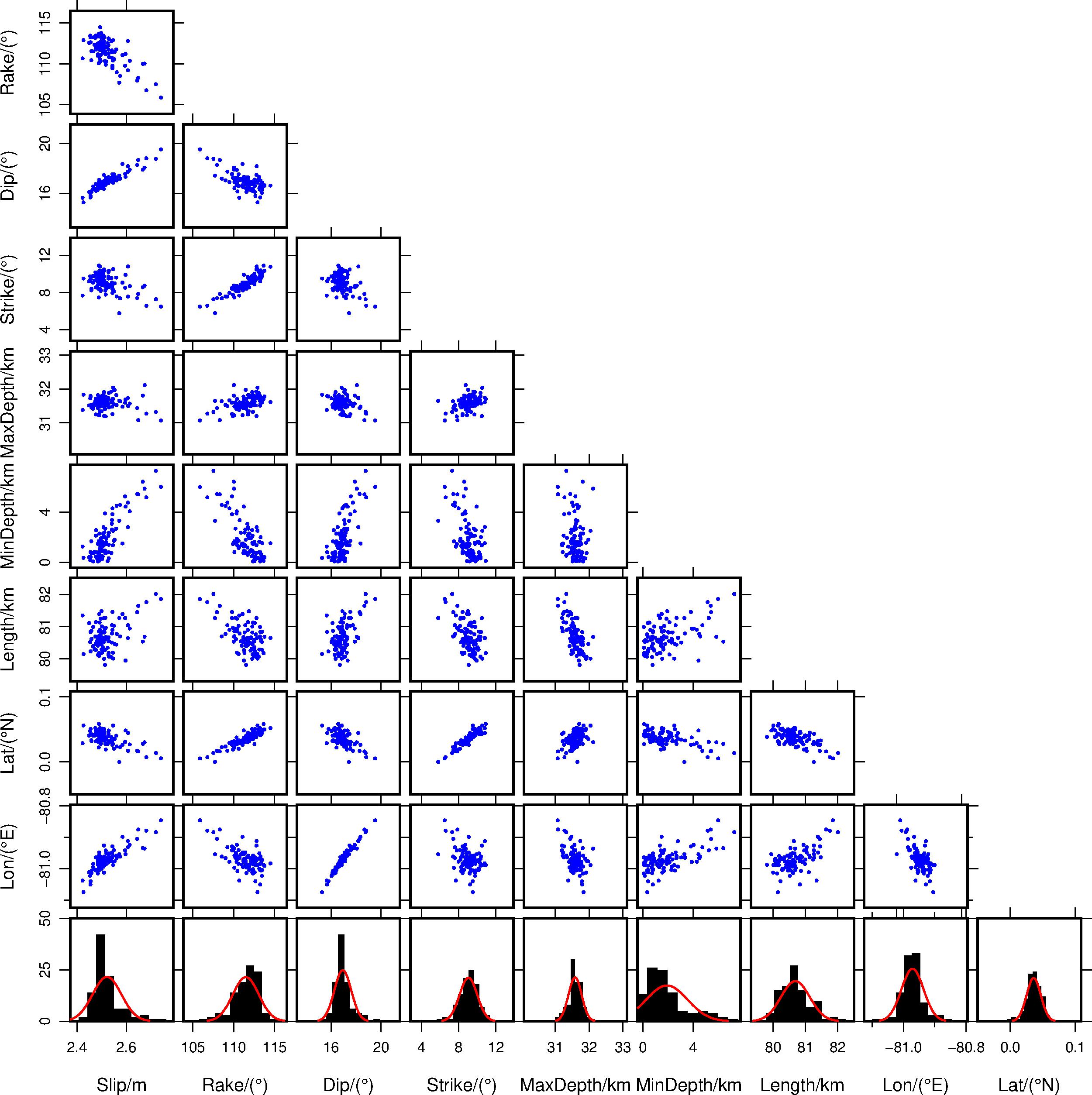
Figure S2 shows the solutions obtained in the nonlinear inversion strategy of Clarke et al. (1997), starting from 100 random initial models. In this inversion, we assume uniform slip over a rectangular fault plane and solve for the location of the center of the surface projection of the fault, fault strike, dip, length, depth of the upper and lower edges of the slip patch, slip rake, and slip magnitude.
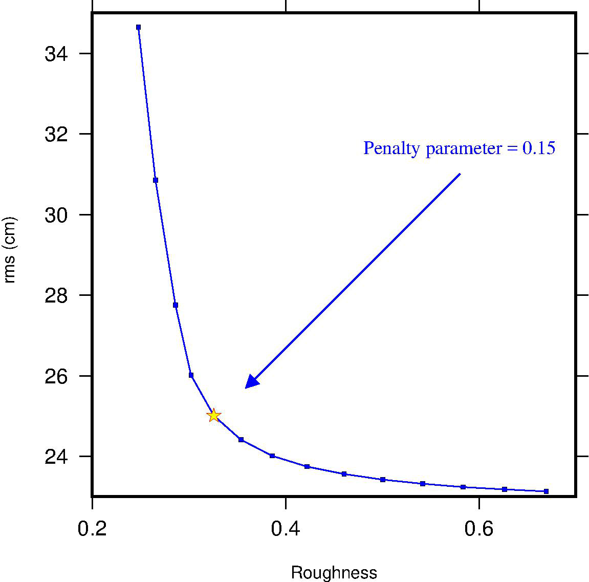
Figure S3 shows the trade-off curve between model roughness and model fit of predicted deformation to observed deformation, for various values of the penalty parameter used in the linear inverse solution for slip distribution, assuming a fault strike of 26°.
Figure S4 corresponds to Figure 4 in the main article, although it shows the predicted and residual interferograms before unwrapping.
Figures S5 and S6 correspond to Figures 3 and 4 in the main article, although they assume a fault strike of 8.7°, which is the best-fitting strike found in the nonlinear inversion.
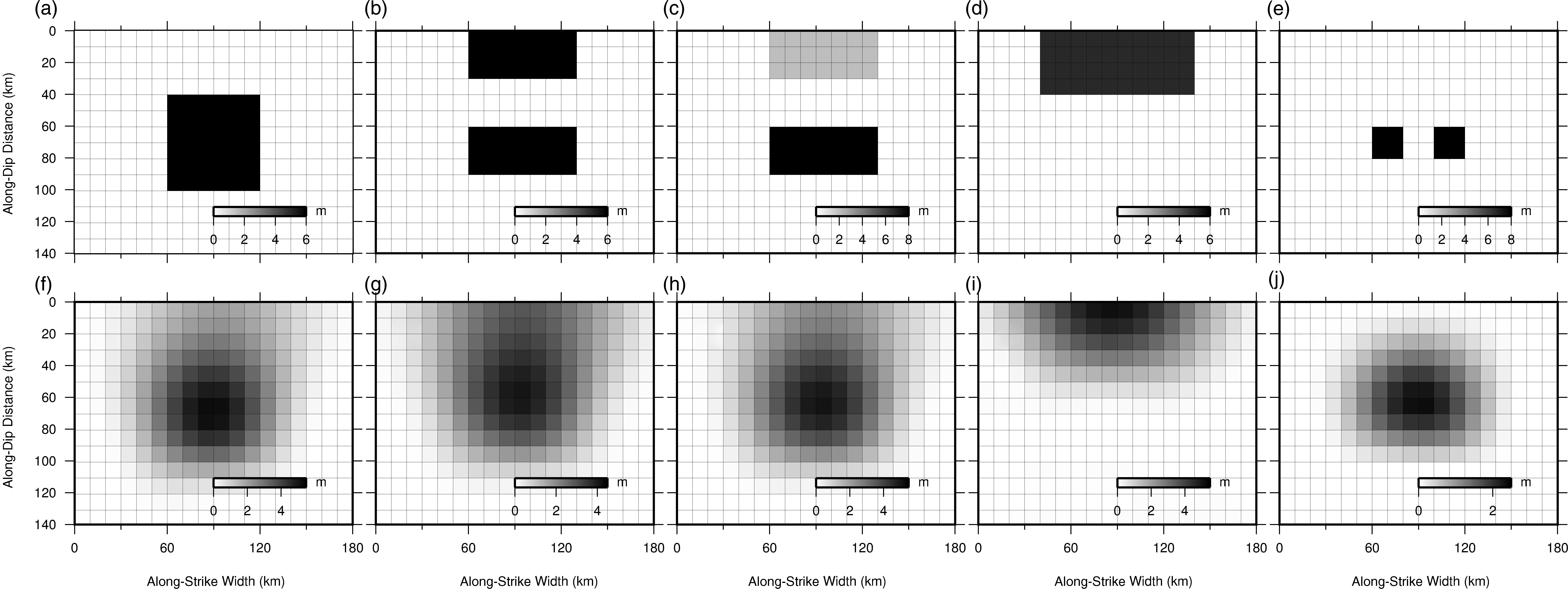
To explore the resolving power of these onshore interferometric data, we construct several idealized slip models. We synthesize interferograms from these slip models, adding noise simulated using the 1D covariance function of the observed interferograms, which we invert for coseismic slip using the same fault plane and regularization penalty parameter as in our preferred model (Fig. S3).
In the first sensitivity test model, there is no slip extending to the trench (Fig. S7a). However, inverting the synthetic interferograms results in inferred slip extending to the trench (Fig. S7f). The inferred slip in this sensitivity test is about half of the magnitude of the near-trench slip in our preferred model (Fig. 3 of the main article). When we include near-trench slip in the synthetic models (Figs. S7b,c), unsurprisingly we also infer near-trench slip when inverting the synthetic interferograms (Figs. S7g,h). Although the onshore geodetic data do have low resolution on the slip near the trench, the larger than slip is, the larger the inferred near-trench slip is when inverting synthetic interferograms, indicating that the near-trench region is not completely unresolved. Indeed, when only near-trench slip is included in the synthetic models (Fig. S7d), the slip inferred by inverting the corresponding synthetic interferograms is indeed constrained only near the trench (Fig. S7i).
To illustrate the effect of the smoothness regularization in our model, Figure S7e shows a model in which coseismic slip is isolated in two distinct patches. Inverting the corresponding synthetic interferogram does not resolve the two distinct slip patches (Fig. S7j). It is important to reiterate that in these sensitivity tests, we use the regularization penalty parameter that was chosen from the L-curve from inverting the real interferogram (Fig. S3). However, this penalty parameter is not necessarily the optimal penalty parameter that would have been chosen if we had constructed L-curves for each of the synthetic tests. In particular, the optimum penalty parameter would be smaller in the synthetic test in Figure S7e if we chose it based on an L-curve analysis specific to these synthetic data, thereby resulting in better resolution of the two distinct slip patches; however, we construct this test to show the ramifications of the smoothness constraint in our preferred model and not to test whether onshore Interferometric Synthetic Aperture Radar (InSAR) data would be able to, in general, resolve two distinct slip patches.
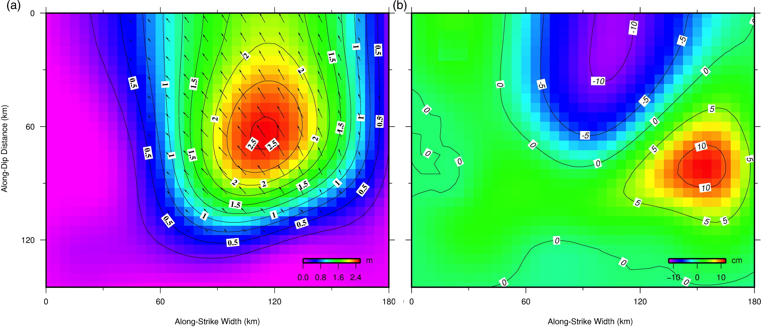
Finally, to illustrate the dependence of the inferred coseismic slip on the assumed elastic structure, we determine a slip model using the same fault geometry as in our preferred model, but assume a layered elastic structure. A four-layer model with parameters referred from CRUST1.0 model (Laske et al., 2013) was used to calculate the Green’s function (the elastic parameters are listed in Table S1). We assume the same regularization penalty parameter as in our preferred model (Fig. S3). Using the layered elastic structure, we infer less slip near the trench (just over 10-cm lower magnitude slip) and slightly more slip extending to the north (Fig. S8).
Table S1. Multilayered crustal model parameters.
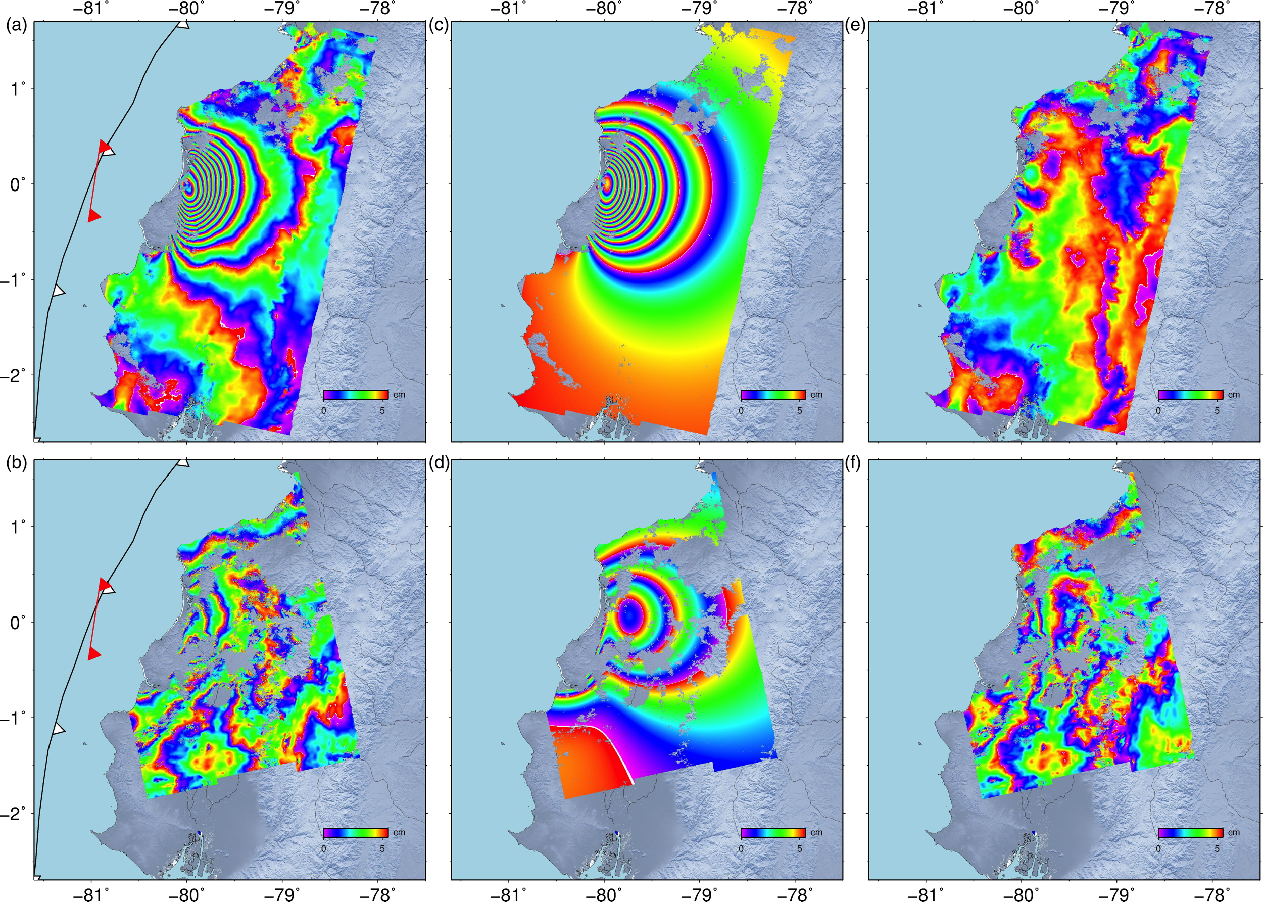
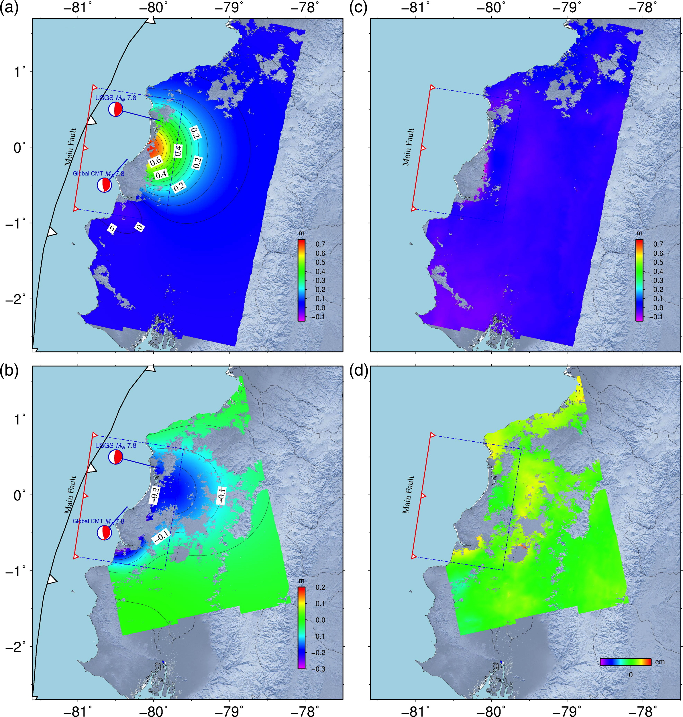
Figure S1. Coseismic interferograms of (a) the descending Sentinel-1A track T040D and (b) the ascending track T018A. Synthetic interferograms on the (c) descending and (d) ascending tracks of the best-fit uniform slip-fault-plane solution. Red barbed line represents the surface trace of the modeled fault plane. Residual interferograms of (e) descending and (f) ascending tracks. Black line is the subduction trench. Each contour on the interferograms indicates a 0.05 m increment in displacement.
Figure S2. Fault parameters determined using 100 random initial models in a nonlinear inversion assuming uniform slip on a rectangular fault patch, shown both in scatter plots and histograms. Red lines are Gaussian probability density functions that best fit the distribution of the individual parameters, rescaled to overplot the histograms.
Figure S3. Trade-off between root mean square (rms) error of predicted-to-observed interferograms and roughness of coseismic slip in the inversion for spatial distribution of coseismic slip in a planar fault for various values of penalty parameters. Optimal penalty parameter (star) is chosen to minimize both rms and roughness.
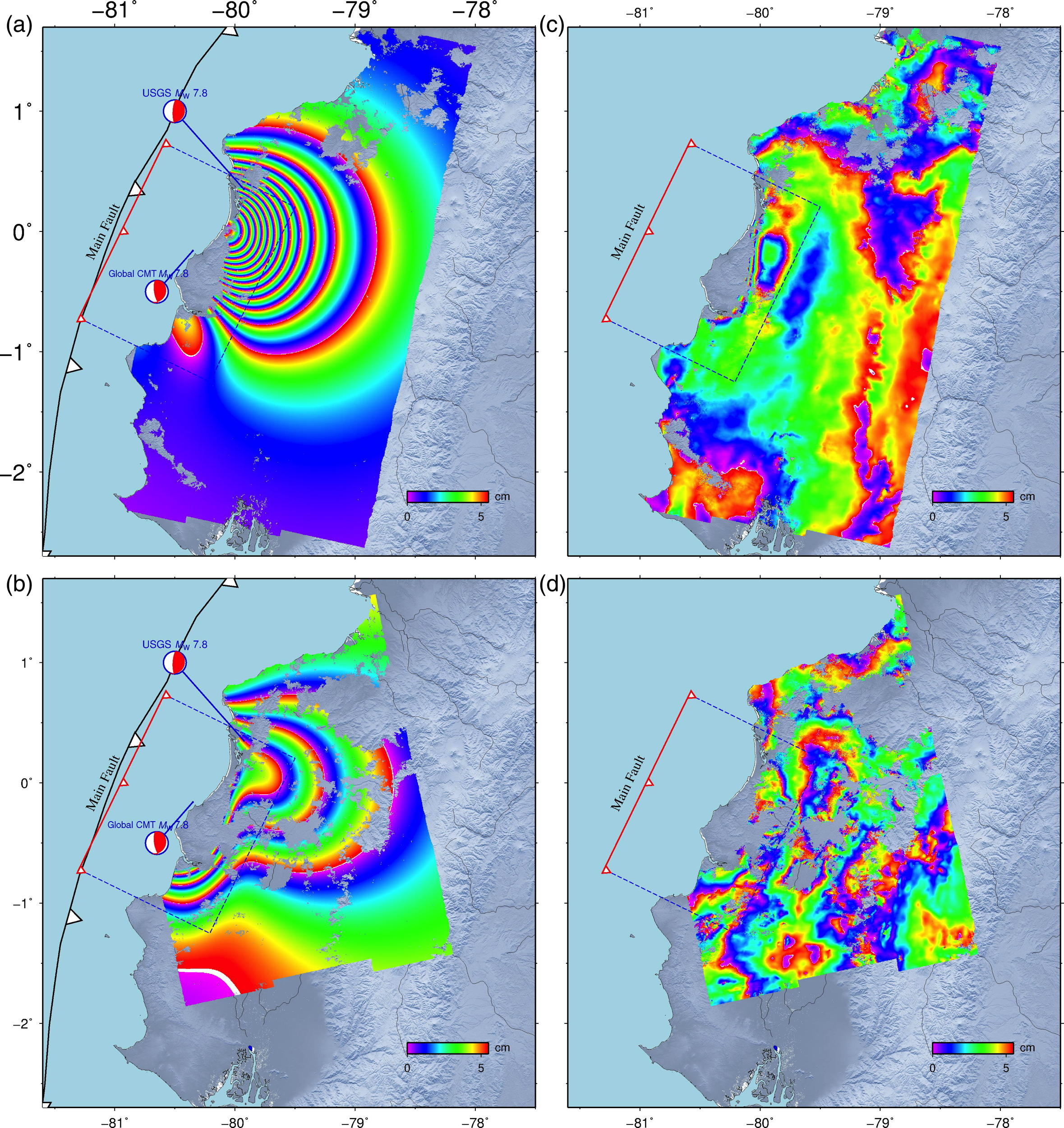
Figure S4. Modeled interferograms for the (a) descending track T040D and (b) ascending track T018A predicted by the slip model in Figure 3a and the associated residuals of the observed interferograms in Figure 2c,d of the main article. The red line is the trace of the model fault plane, and the blue dashed lines represent the surface projections of the modeled fault. Each contour indicates a 0.05 m increment in displacement. Figure S4 is identical to Figure 4 in the main article, except here the interferograms are shown in a wrapped sense.
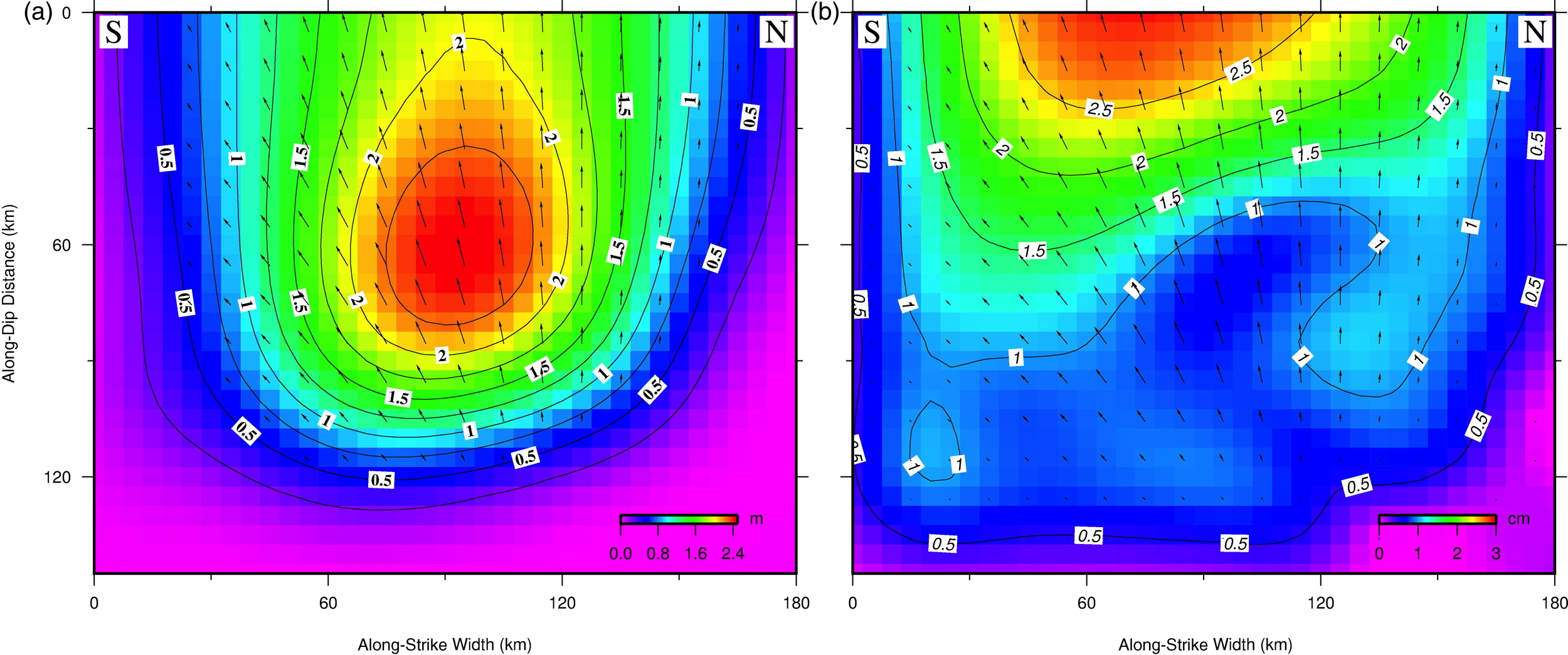
Figure S5. (a) Coseismic slip model determined from the interferograms, assuming a fault location and dip determined in the nonlinear inversion assuming uniform slip and using the fault strike of 8.7°, which is the best-fitting strike found in the nonlinear inversion assuming uniform slip. Arrows show the sense of motion of the hanging wall, and contours are labeled in meters. (b) Standard deviation of coseismic slip inferred in the Monte Carlo estimation with 100 perturbed datasets.
Figure S6. Modeled interferograms for the (a) descending track T040D and (b) ascending track T018A predicted by the slip model in Figure S5a and the associated residuals of the observed interferograms in Figure 2c,d of the main article. The red line is the trace of the model fault plane, and the blue dashed lines represent the surface projections of the modeled fault. Each contour indicates a 0.05 m increment in displacement.
Figure S7. (a–e) Synthetic slip models used in sensitivity, and (f–j) slip inferred by inverting synthetic interferograms corresponding to the slip model above each panel, assuming the fault geometry and optimum penalty parameter in our preferred coseismic slip model.
Figure S8. (a) Coseismic slip determined from the interferogrametric data, assuming the fault geometry used in our preferred model (Fig. 3 of the main article), although assuming a layered elastic structure. Arrows show the sense of motion of the hanging wall, and contours are labeled in meters. (b) Difference between the coseismic slip in (a) and our preferred model (Fig. 3 of the main article), which assumed a homogeneous elastic structure.
Download: Slip_model_pre [Zipped Plain Text Space-delimited Values; ~7 KB]. This file contains the preferred slip model data used in this study.
Clarke, P. J., D. Paradissis, P. Briole, P. C. England, B. E. Parsons, H. Billiris, and J. C. Ruegg (1997). Geodetic investigation of the 13 May 1995 Kozani-Grevena (Greece) earthquake, Geophys. Res. Lett. 24, no. 6, 707–710.
Laske, G., G. Masters, Z. Ma, and M. Pasyanos (2013). Update on CRUST1.0—A 1-degree global model of Earth's crust, Geophys. Res. Abstr. 15, Abstract EGU 2013-2658.
[ Back ]