This electronic supplement contains tables and figures showing alternative fault-slip models and results of the Sentinel-1 time-series analysis. Figure S1 shows an estimate of uncertainty on the preferred fault-slip model from our Markov chain Monte Carlo (MCMC) analysis. The details of alternative slip model for the Pawnee mainshock allowing both strike- and dip-slip motion (Fig. S2), data fit for the alternative slip model (Fig. S3), and probability density functions for the smoothing factors of the alternative slip model (Fig. S4) from our MCMC analysis are shown. Another alternative slip model for the Pawnee mainshock constrained to strike-slip motion on a fault plane limited to 12 km depth instead of the 15 km model fault width of Figure 5 (in the main article) and Figure S1 (Fig. S5) and data fits for the narrow-fault model (Fig. S6) are also described. The difference in the synthetic surface deformation predicted by the preferred wide-fault and the narrow-fault model projected into the three radar line-of-sight (LoS) directions (Fig. S7) is also shown. The outputs of the Generic Interferometric Synthetic Aperture Radar (InSAR) Analysis Toolbox (GIAnT) time-series analysis (Agram et al., 2013) of the Sentinel-1A/1B InSAR data from July 2015 to November 2016, including the step function, linear rate, constant, and seasonal terms along with their associated error estimates from the jackknife analysis (xval in GIAnT; Figs. S8–S16) are also given.
Table S1 [Plain text comma-separated values; ~105 KB]. Relocated hypocentral locations for events in the Pawnee area.
Table S2. List of interferograms processed.
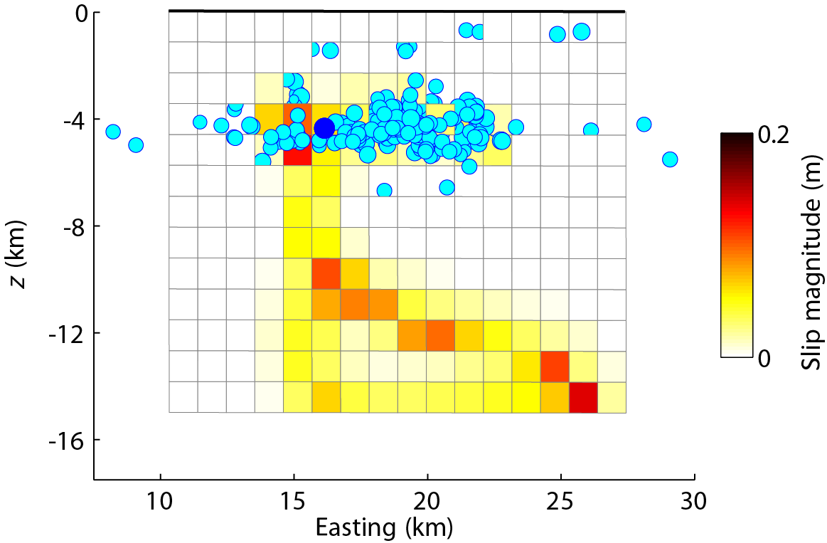
Figure S1. Estimate of the uncertainty in the preferred fault-slip model of Figure 5 (in the main article) on vertical plane, viewed from south. Estimate calculated from standard deviation of slip on each patch in the set of kept models in Markov chain Monte Carlo (MCMC) optimization, which reflects uncertainty due to variations in the strength of the smoothing function but not uncertainty due to noise in the data or Earth model parameters.
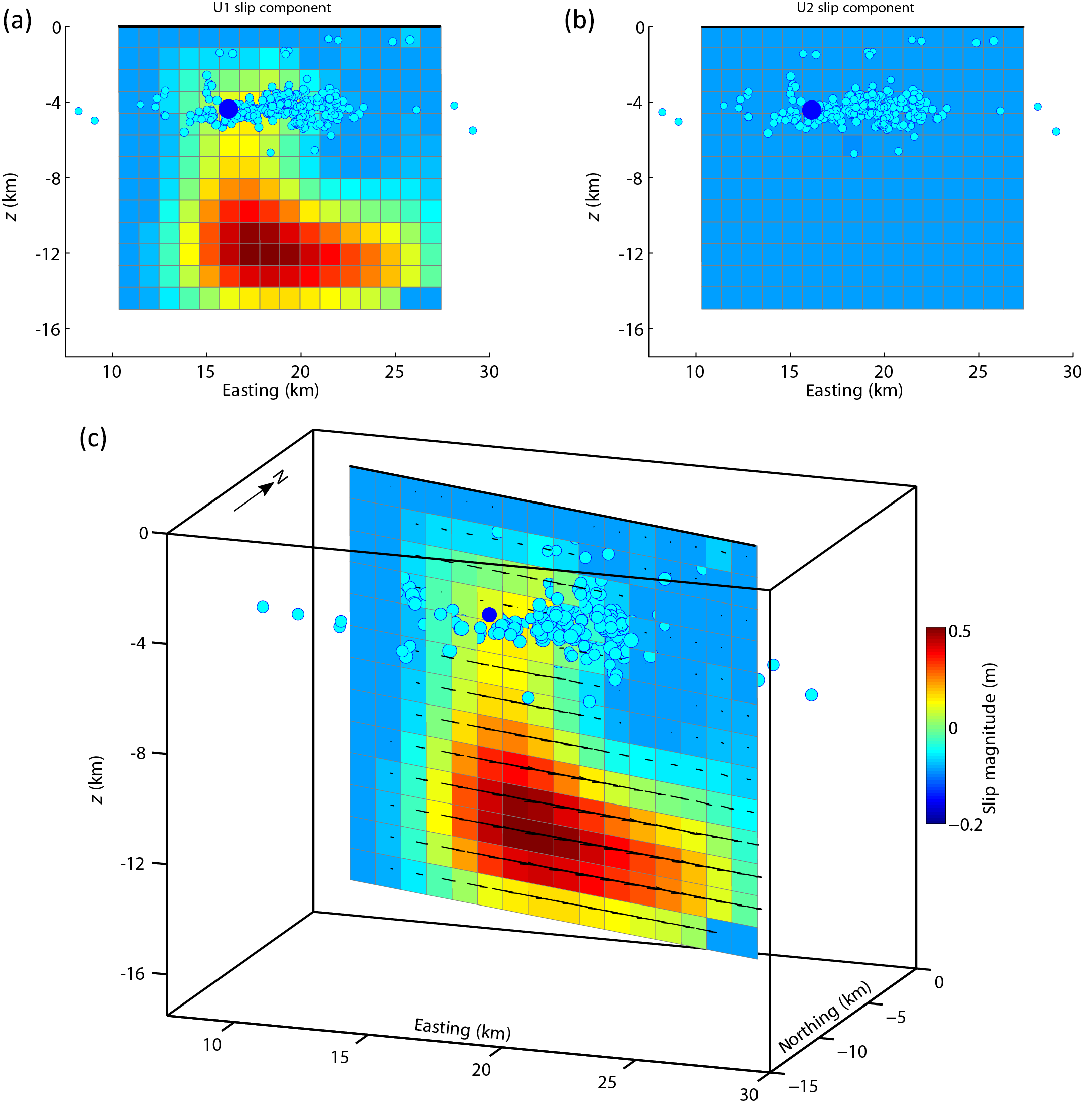
Figure S2. Static fault-slip model for Pawnee mainshock, similar to Figure 5 in the main article, but with both strike-slip and dip-slip motion allowed. Slip on patches where uncertainty is greater than the value has been set to zero. (a) Slip model strike-slip component distribution on vertical plane, viewed from south. (b) Slip model dip-slip component distribution on vertical plane, viewed from south. (c) Perspective view of slip distribution from southwest. Arrows show magnitude and direction of motion of southern block relative to northern block.
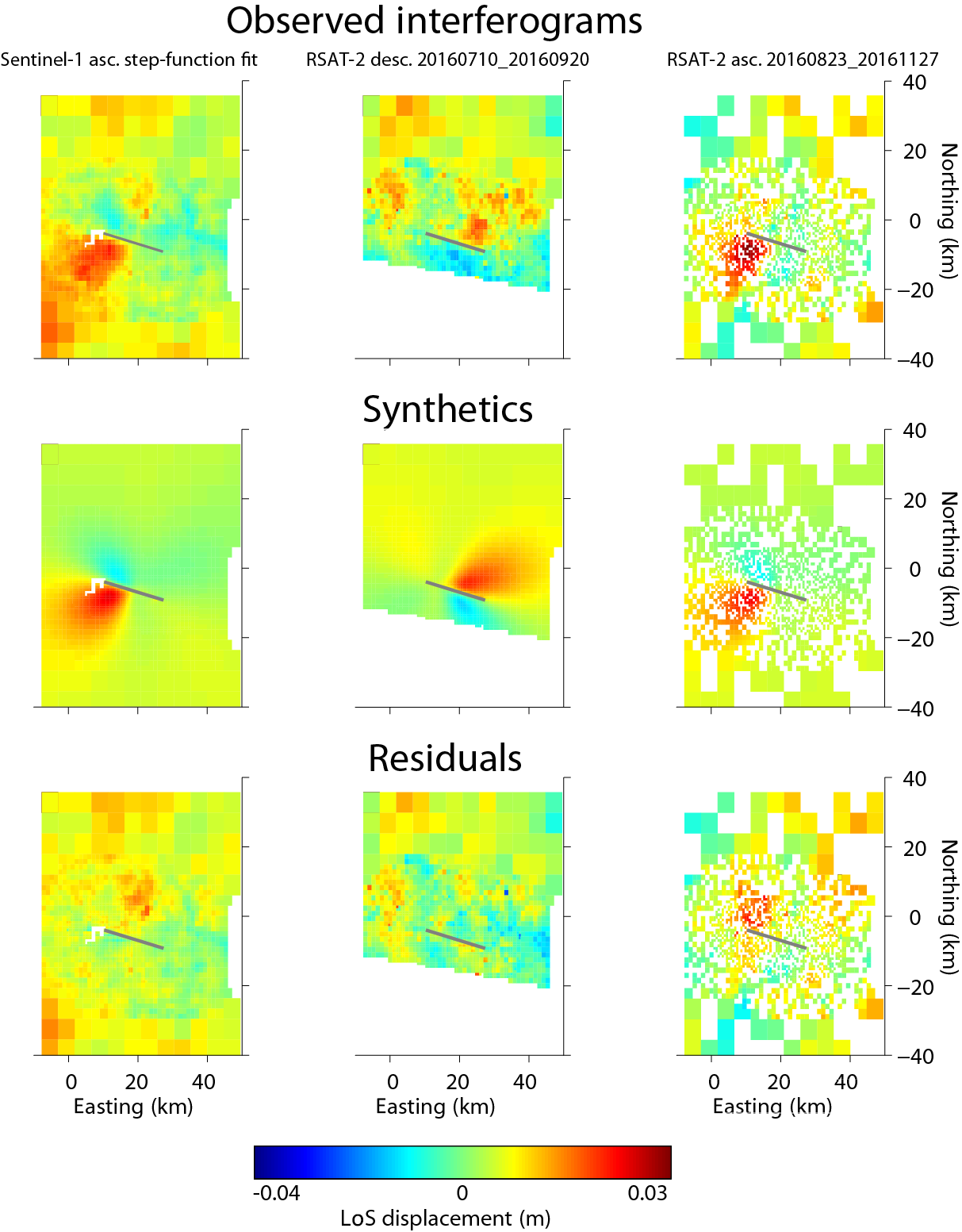
Figure S3. Maps of downsampled interferogram data (top row), alternative slip model prediction or synthetic (middle row), and residuals (bottom row), all with same color scale, similar to Figure 6 of the main article. Columns are three InSAR datasets: left is Sentinel-1 time-series coseismic step, middle is RADARSAT-2 descending track, and right is RADARSAT-2 ascending track. Motion in LoS direction on these plots is positive away from the satellite.
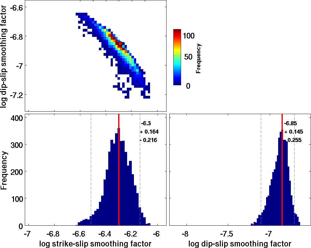
Figure S4. Histograms or probability density function maps of smoothing factors for alternative slip model from 5000 MCMC runs. Top shows 2D scattergram of dip-slip and strike-slip factors. The most probable value used in solution shown in Figures S2 and S3 is marked with a red-filled black outline circle. Bottom panels are individual 1D histograms. Base 10 logarithms of smoothing factors are shown. The smaller number (more negative log) for the dip-slip smoothing factor means greater smoothing for that component was more optimal.
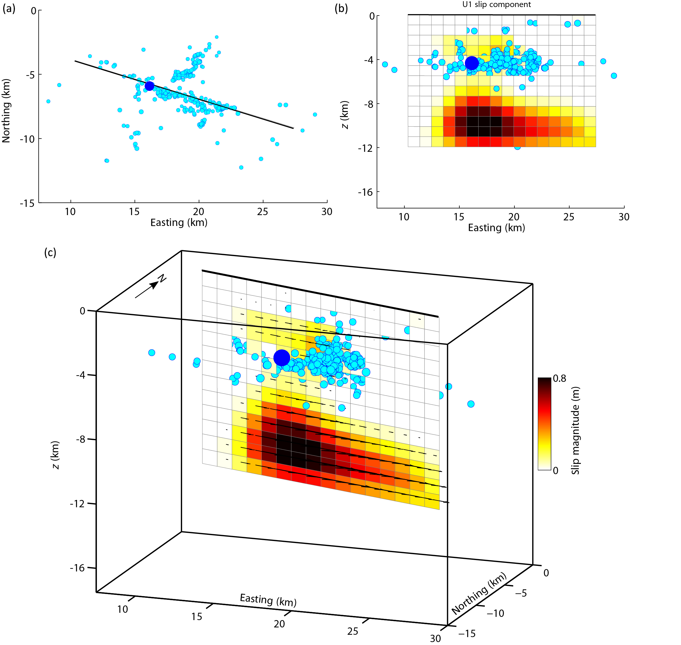
Figure S5. Static fault-slip model for Pawnee mainshock, similar to Figure 5 in the main article, but with model fault limited to 12 km depth. Slip on patches where uncertainty is greater than the value has been set to zero. (a) Map view of model fault location in local Cartesian coordinate system (kilometers relative to 36.4788° N, −97.1144° E). (b) Slip model strike-slip component distribution on vertical plane, viewed from south. (c) Perspective view of slip distribution from southwest. Arrows show magnitude and direction of motion of southern block relative to northern block.
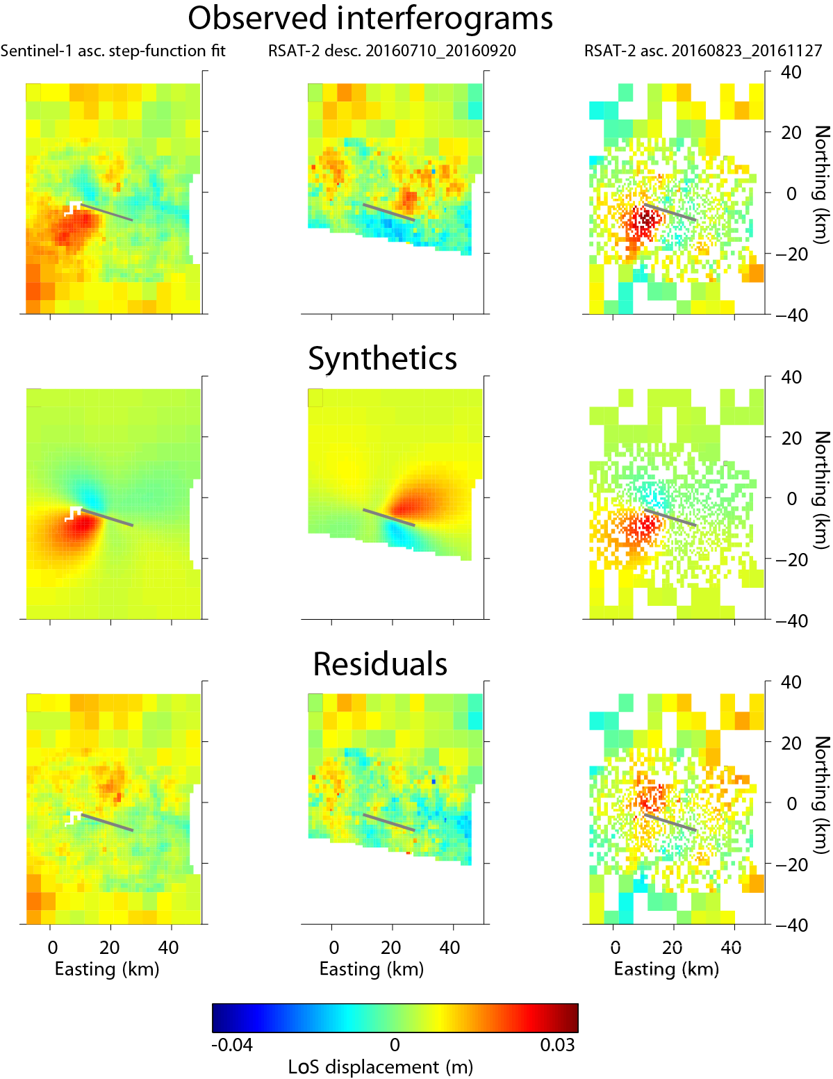
Figure S6. Maps of downsampled interferogram data (top row), alternative slip model prediction or synthetic from narrow-fault model (middle row), and residuals (bottom row), all with same color scale, similar to Figure 6 of the main article. Columns are three InSAR datasets: left is Sentinel-1 time-series coseismic step, middle is RADARSAT-2 descending track, and right is RADARSAT-2 ascending track. Motion in LoS direction on these plots is positive away from the satellite.
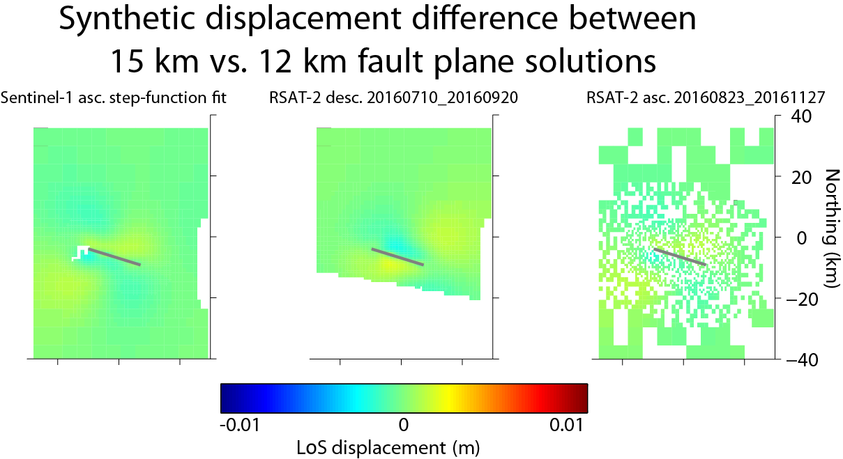
Figure S7. Map of difference between synthetic or model prediction from narrow-fault model (Figs. S4 and S5) and the preferred slip model (Figs. 5 and 6 in the main article) projected into the LoS directions of the three InSAR datasets. Columns are three InSAR datasets: left is Sentinel-1 time-series coseismic step, middle is RADARSAT-2 descending track, and right is RADARSAT-2 ascending track. Motion in LoS direction on these plots is positive away from the satellite.
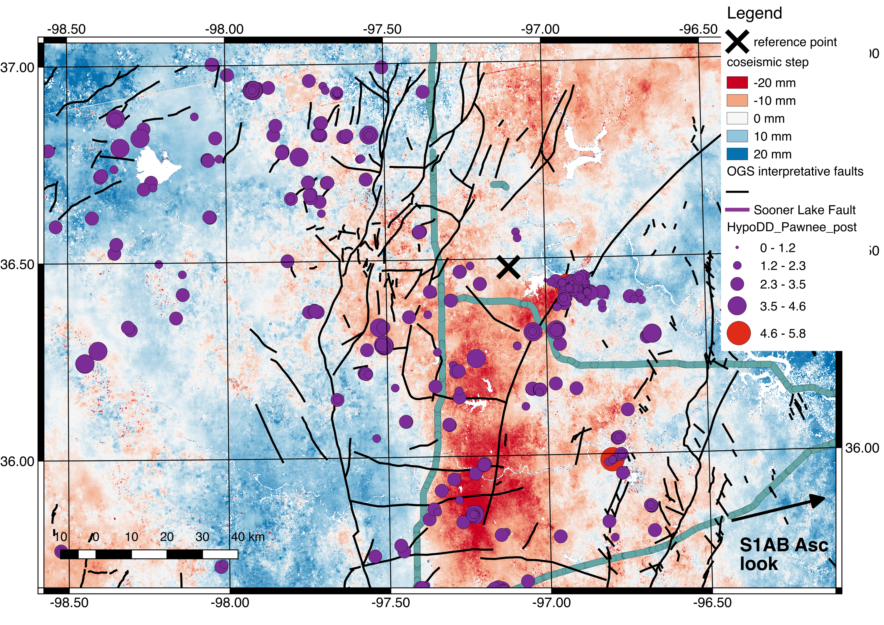
Figure S8. GIAnT step function fit to Sentinel-1A/1B time series through 2 November for Pawnee mainshock coseismic LoS deformation estimate, similar to Figure 4 in the main article but for larger area. Large black X symbol marks the location of reference point for time-series analysis. Black lines are interpretive faults from Oklahoma Geological Survey fault database (Marsh and Holland, 2016). Magenta line is our model fault location. Circles filled with purple (magnitude < 4.6) and red (magnitude > 4.6) show hypoDD relocated earthquakes after the Pawnee earthquake through 14 November 2016. Map is in Universal Transverse Mercator (UTM) zone 14 projection.
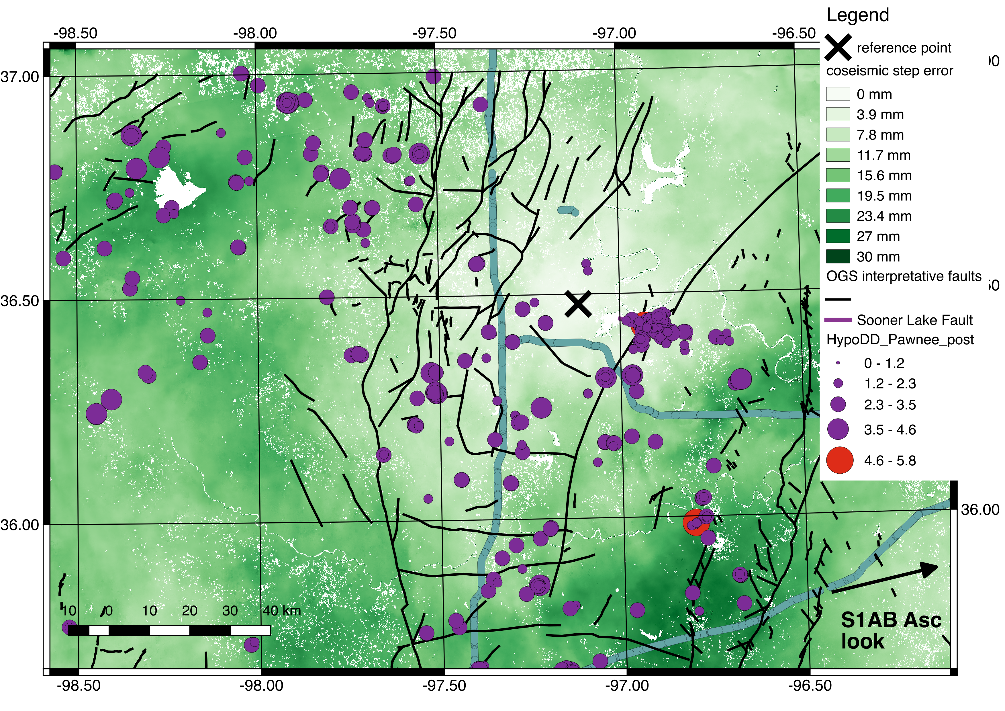
Figure S9. GIAnT step function fit error estimate from Sentinel-1A/1B time series for Pawnee mainshock coseismic LoS deformation. Other symbols as in Figure S4.
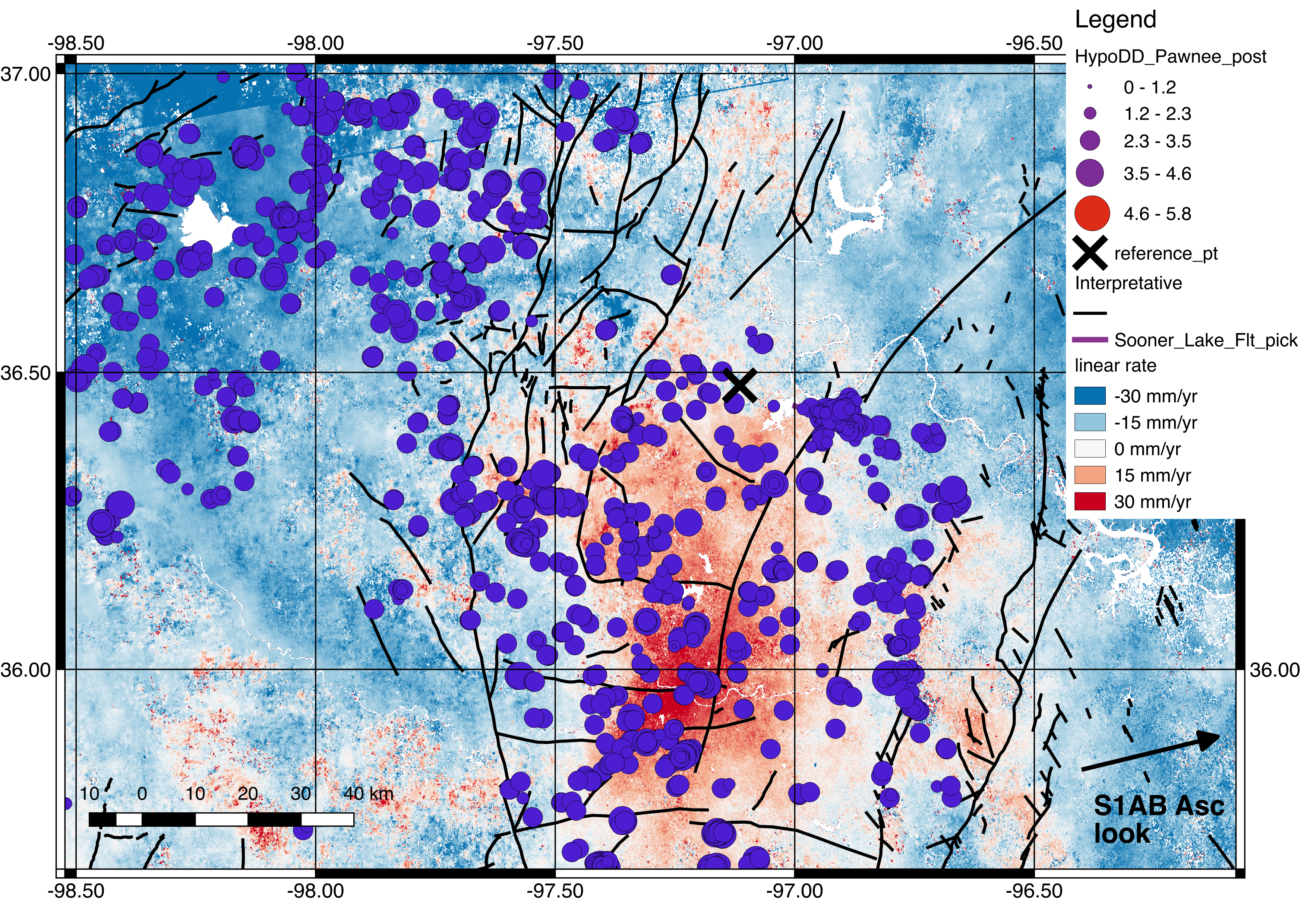
Figure S10. GIAnT linear rate fit to Sentinel-1A/1B time series 23 July 2015 through 2 November 2016. Other symbols as in Figure S4.
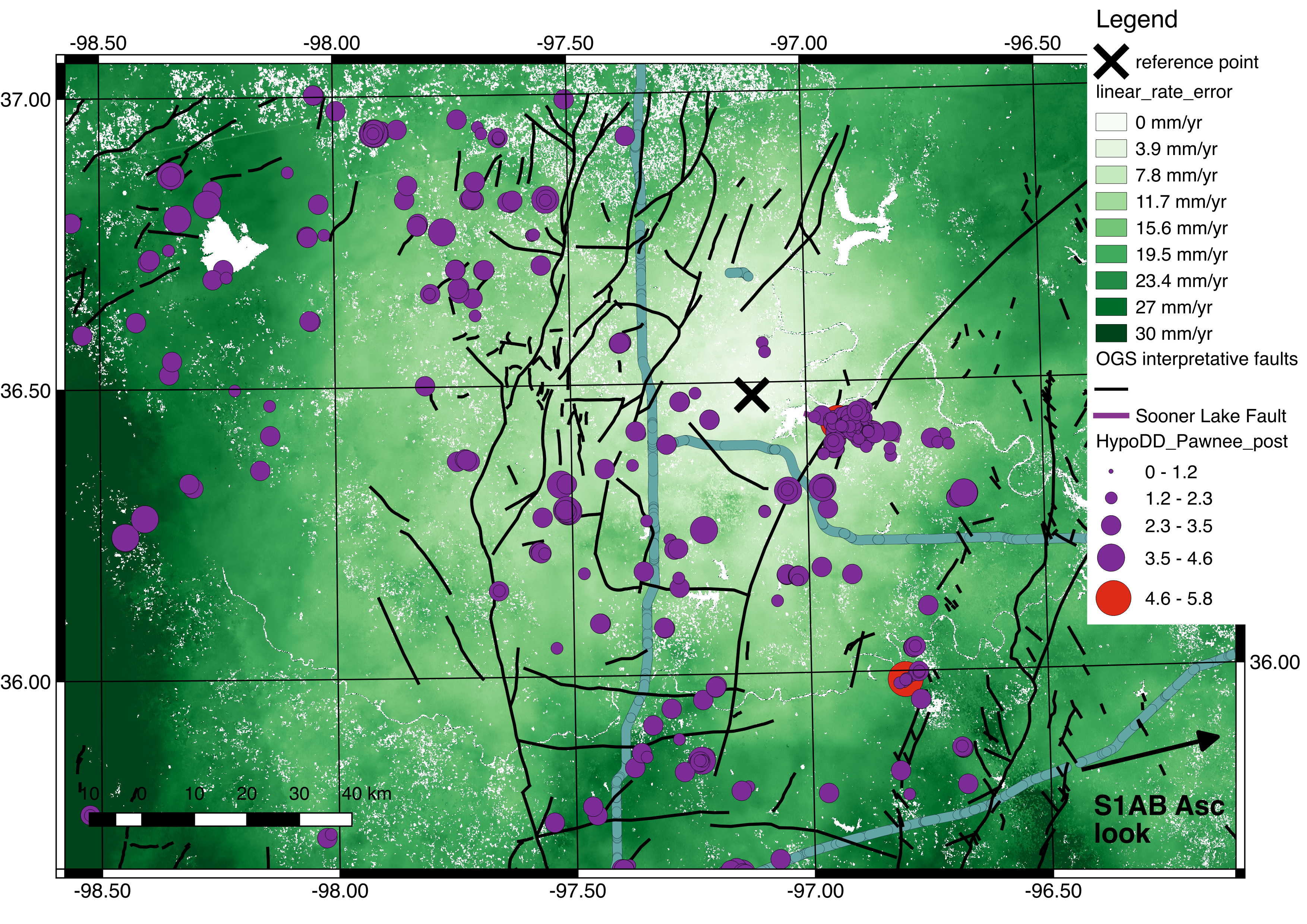
Figure S11. GIAnT linear rate error estimate from Sentinel-1A/1B time series 23 July 2015 through 2 November 2016. Other symbols as in Figure S4.
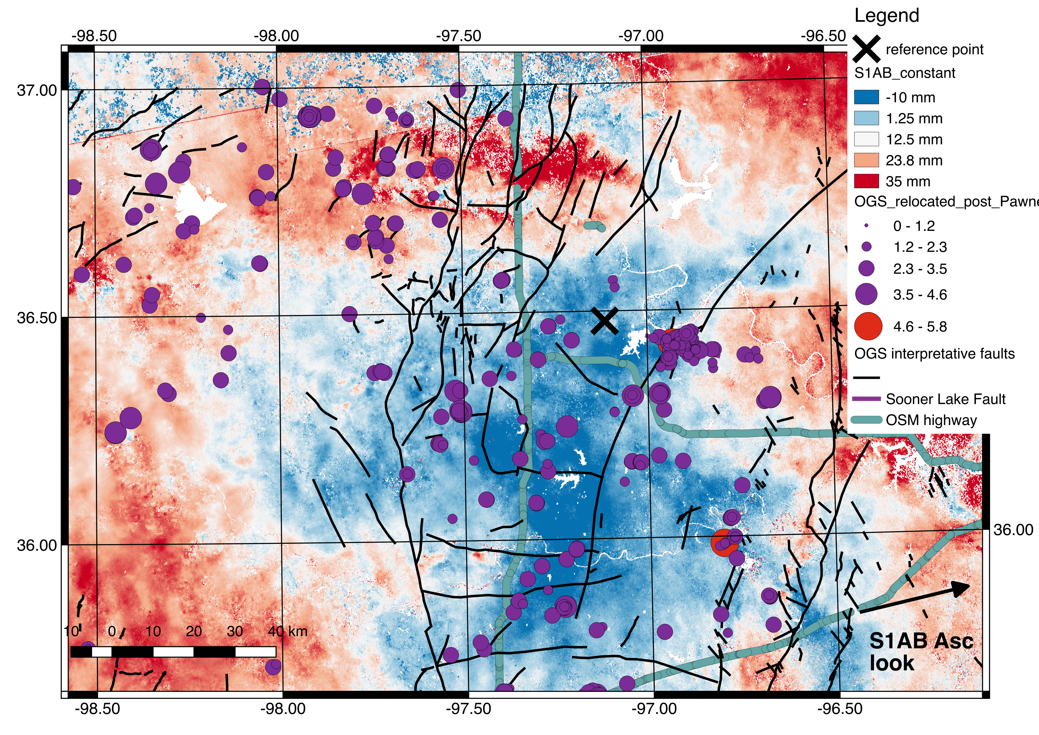
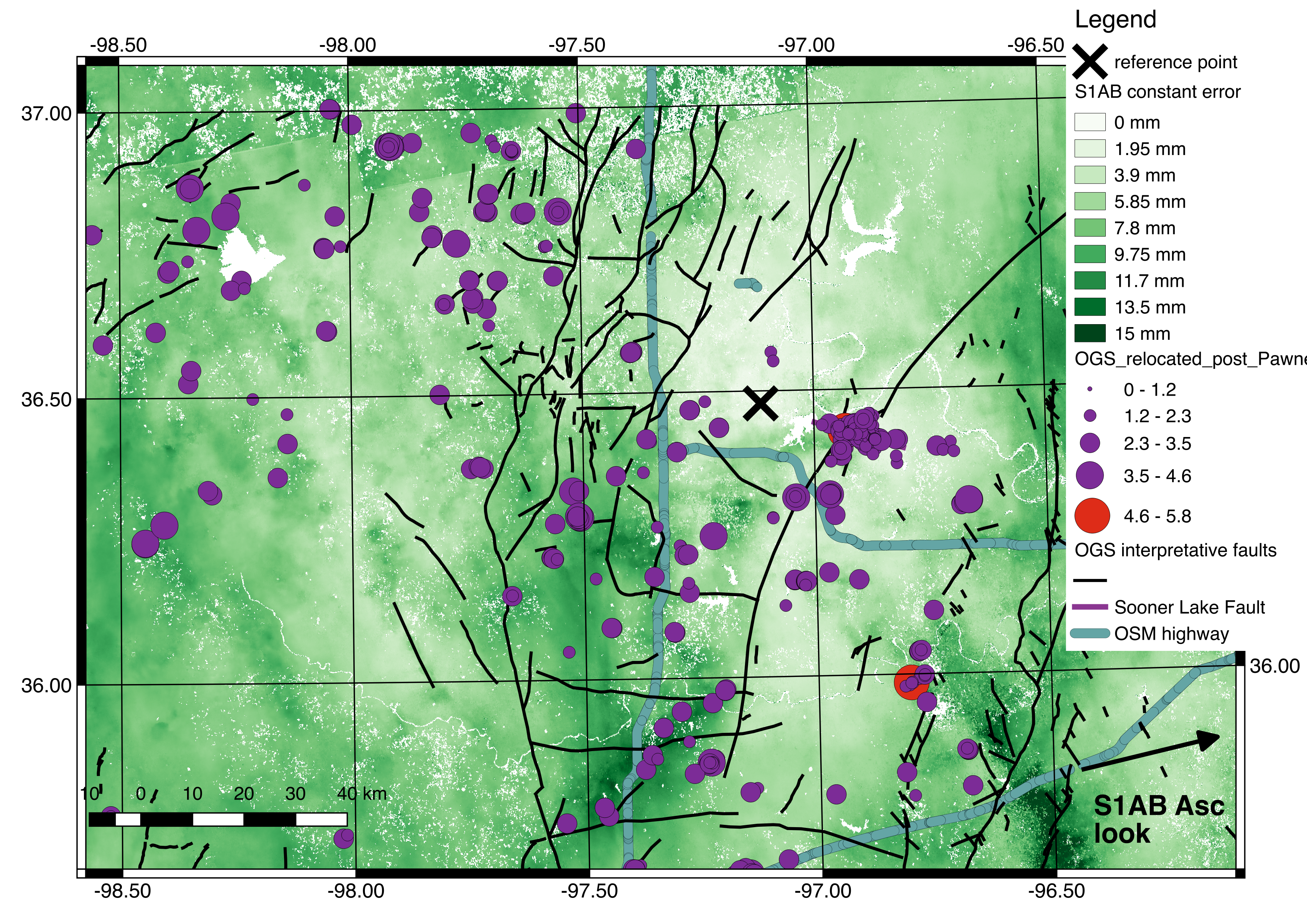
Figure S12. GIAnT constant term from fit to Sentinel-1A/1B time series 23 July 2015 through 2 November 2016, largely due to atmosphere in the reference date that is first date of series. Other symbols as in Figure S4.
Figure S13. GIAnT constant term error estimate for fit to Sentinel-1A/1B time series 23 July 2015 through 2 November 2016, largely due to atmosphere in the reference date that is first date of series. Other symbols as in Figure S4.
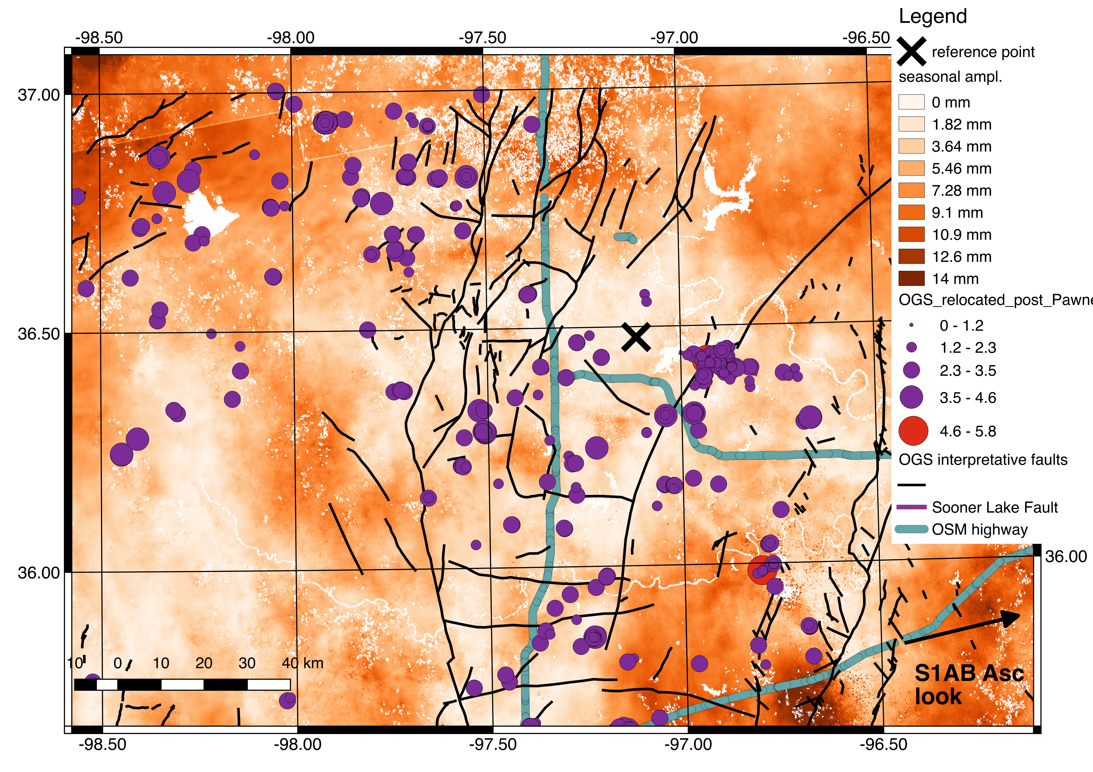
Figure S14. GIAnT amplitude of seasonal terms from fit to Sentinel-1A/1B time series 23 July 2015 through 2 November 2016. The seasonal cosine and sine terms have been combined to estimate the seasonal amplitude in this plot. Other symbols as in Figure S4.
Figure S15. GIAnT amplitude of seasonal terms error estimate for fit to Sentinel-1A/1B time series 23 July 2015 through 2 November 2016. The seasonal cosine and sine terms have been combined to estimate the error of seasonal amplitude in this plot. Other symbols as in Figure S4.
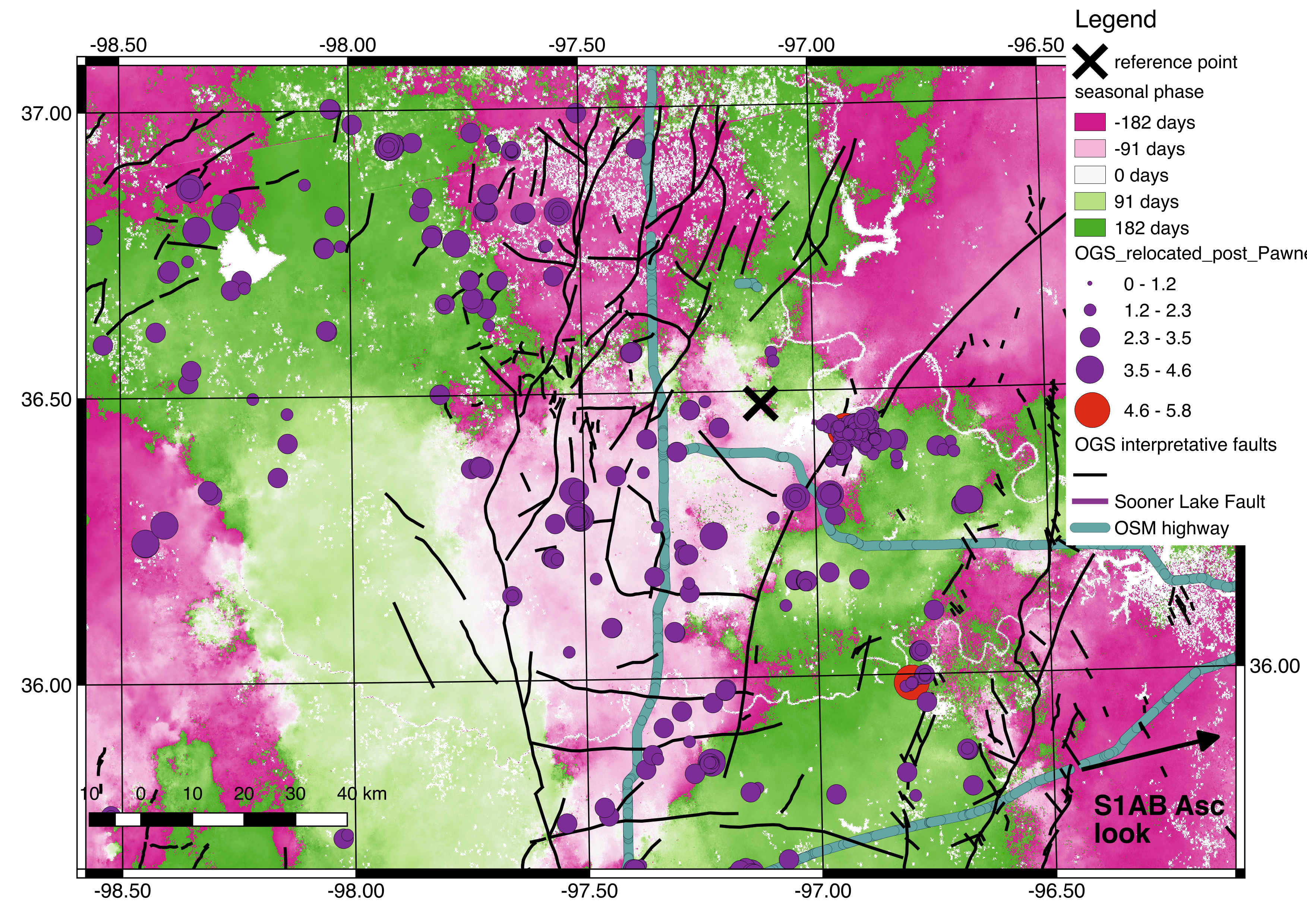
Figure S16. GIAnT amplitude of seasonal term from fit to Sentinel-1A/1B time series 23 July 2015 through 2 November 2016. The seasonal cosine and sine terms have been combined to estimate the phase of the seasonal signal in this plot. Other symbols as in Figure S4.
Agram, P. S., R. Jolivet, B. Riel, Y. N. Lin, M. Simons, E. Hetland, M. P. Doin, and C. Lasserre (2013). New radar interferometric time series analysis toolbox released, Eos Trans. AGU 94, 69–70.
Marsh, S., and A. Holland (2016). Comprehensive fault database and interpretive fault map of Oklahoma, Oklahoma Geol. Surv. Open-File Rept. OF2-2016, Oklahoma Geological Survey, Norman, Oklahoma, 15 pp.
[ Back ]