This electronic supplement contains table of relocated seismicity, ascending orbit interferograms, and figures of slip inversion results.
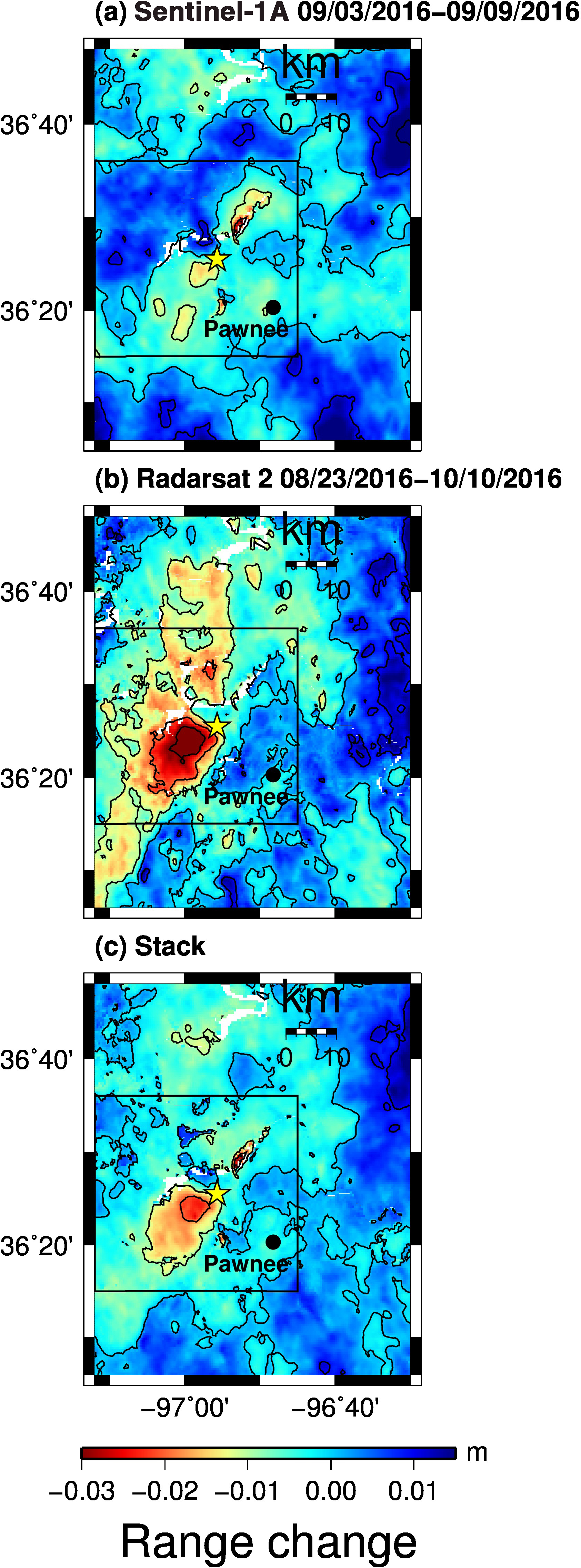
Two ascending orbit interferograms and their stack presented in Figure 2 of the main article exhibit southwest quadrant line-of-sight (LoS) displacement of ~−2.5 cm and a subdued (~+0.5 cm) northwest quadrant LoS displacement. We processed two additional interferograms spanning the mainshock with relatively high coherence and short perpendicular baselines. These are a Sentinel-1A ascending orbit interferogram (Fig. S1a) and a Radarsat 2 ascending orbit interferogram (Fig. S2a). Although the relative amplitude of the western quadrants varies between the two interferograms, their stack (Fig. S2c) exhibits a much stronger amplitude in the southwest quadrant relative to the northwest quadrant LoS displacement, similar to the stacked interferogram that was used in the dislocation modeling (Fig. 2c of the main article).
Relocated seismicity in northcentral Oklahoma includes relocations of seismicity cataloged by the Oklahoma Geological Survey (OGS) as well as newly detected events based on seismic data recorded up to three months after the 3 September 2016 mainshock. The hypoDD relocated seismicity for the Pawnee sequence, shown in Figures 1, 4, and 5 of the main article, is presented in Table S1.
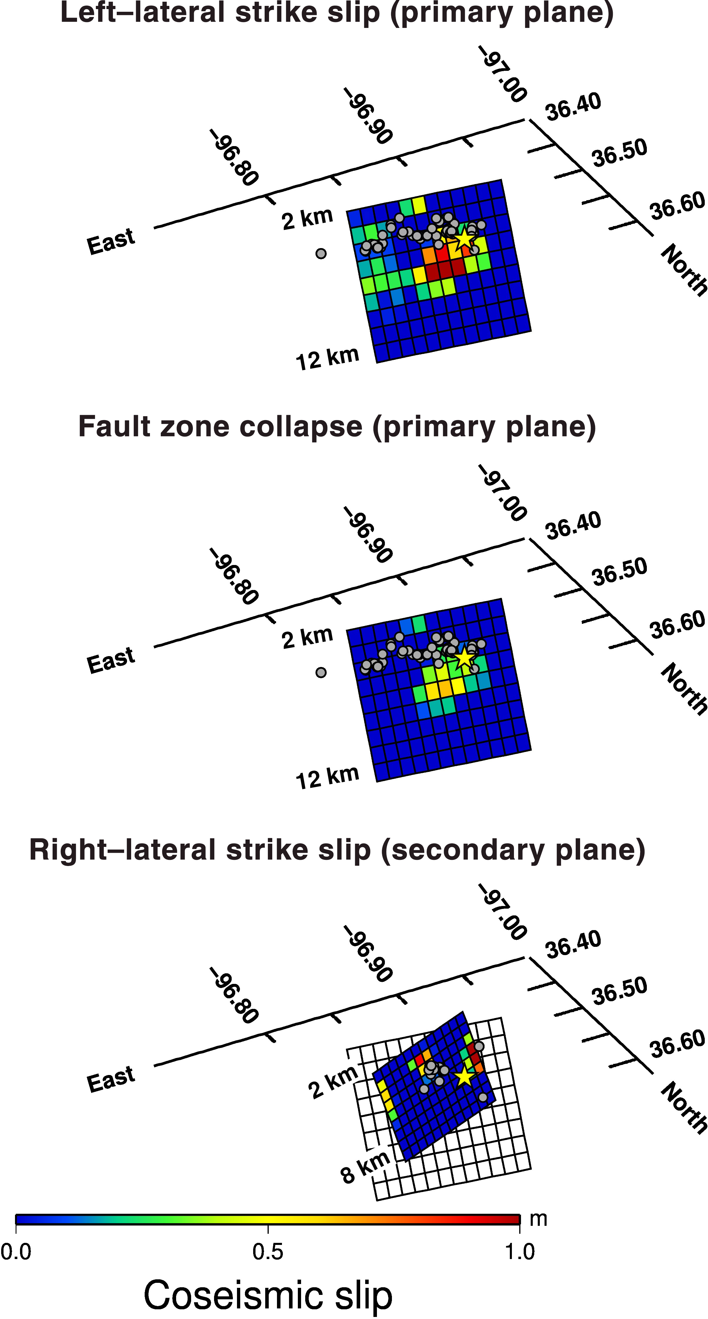
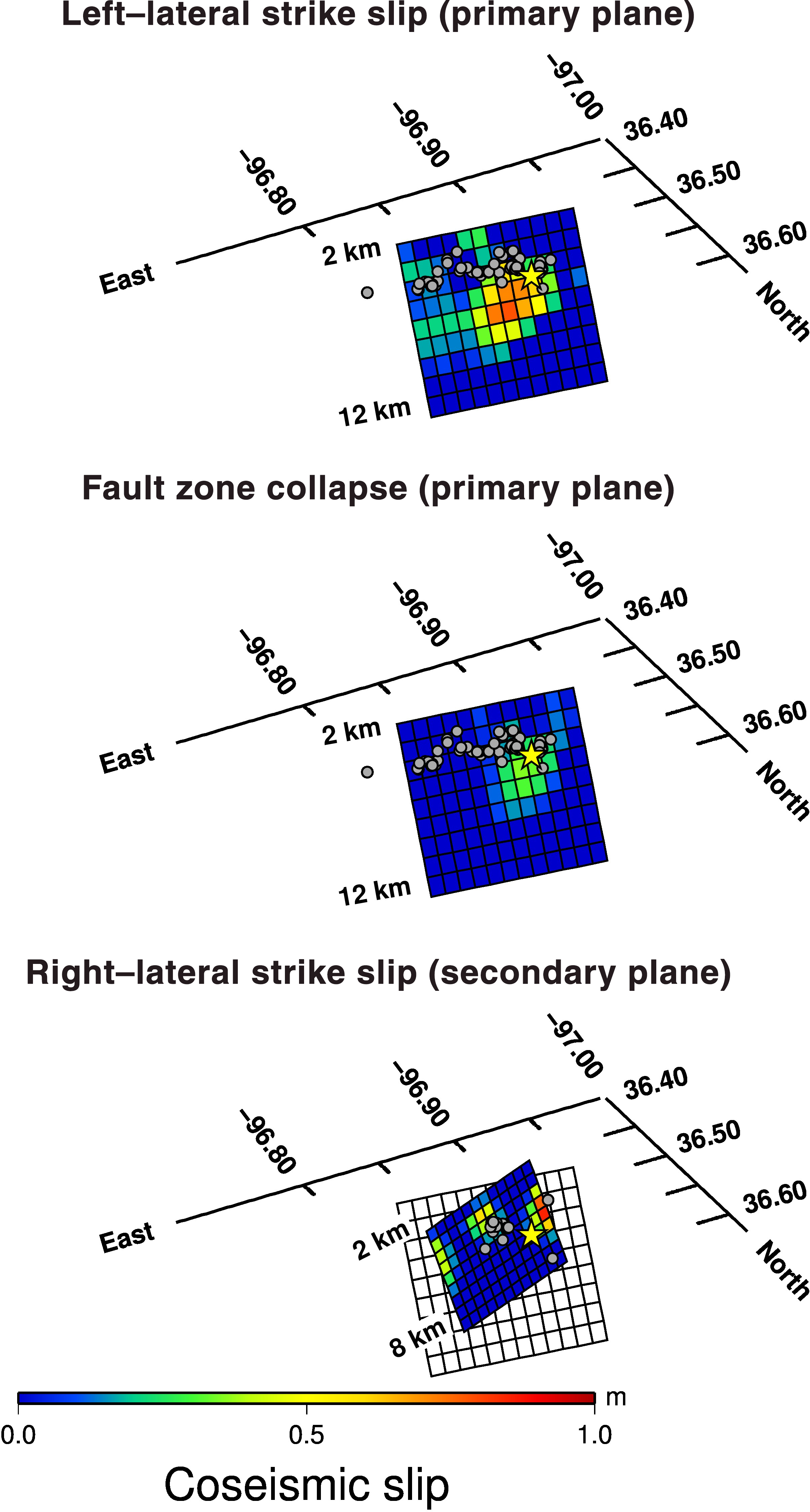
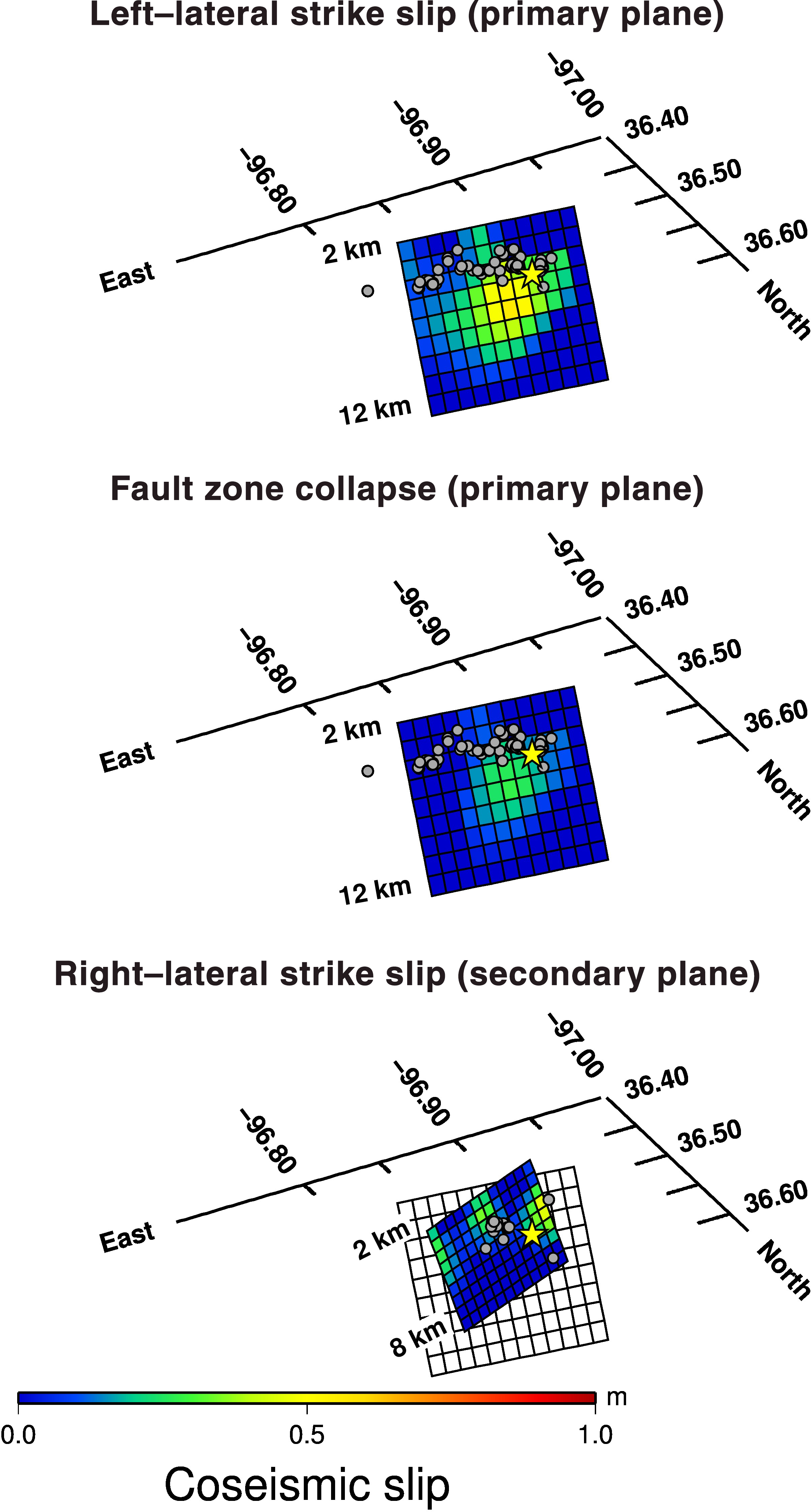
Our simulated annealing method for determining slip distributions from Global Positioning System (GPS) and Interferometric Synthetic Aperture Radar (InSAR) data is effective in deriving an optimal slip distribution but not for assessing model errors. A more comprehensive approach would be to sample a large model space (e.g., Monte Carlo Markov Chain methods) and assess the variance of the best-fitting models. Here, we sample a small part of the model space for model C (which includes fault-zone collapse on the primary plane and afterslip on the secondary plane, i.e., Table 2 of the main article) by varying the smoothing weights from a factor of ¼ to 4 relative to the reference set of smoothing weights employed in the Coseismic Slip Inversion section of the main article. The resulting slip distributions are shown in Figures S2, S3, and S4.
Table S1 [Plain text comma-separated values; ~24 KB]. The relocated hypocenters from 288 Mw ≥1.0 events over the period 1 August 2016 to 22 November 2016. Id, earthquake ID from OGS; Lat, latitude (°); lon, longitude (°); depth, depth from surface (km); year, origin time, year; month, origin time, month; day, origin time, day; hour, origin time, hour; minute, origin time, minute; second, origin time, second; mag, magnitude, from OGS catalog; nccp, number of cross-correlated P-wave differential times; nccs, number of cross-correlated S-wave differential times; nctp, number of catalog P-wave differential times; ncts, number of catalog S-wave differential times; rcc, root mean square (rms) residual for cross-correlated differential times; rct, rms residual for catalog differential times.
Figure S1. (a) Unwrapped Sentinel-1A interferogram covering 3 September 2016 (11 hrs before the mainshock) to 9 September 2016. The heading and incidence angle are 350.1° and 41.3° E. (b) Unwrapped Radarsat 2 interferogram covering 23 August 2016 to 10 October 2016. The heading and incidence angle are 349.9° and 39.6° E. (c) Stack of the two interferograms. The yellow star denotes the National Earthquake Information Center (NEIC) epicenter.
Figure S2. The model C slip distribution obtained using a set of smoothing weights equal to ¼ the weights of the reference set.
Figure S3. The model C slip distribution obtained using a set of smoothing weights equal to the weights of the reference set. This is identical to Figure 9 of the main article.
Figure S4. The model C slip distribution obtained using a set of smoothing weights equal to four times the weights of the reference set.
[ Back ]