The following files contain: (1) Figures S1-S4, which show the unwrapped interferograms modeled in the main text, the quadtree sampling of the interferograms, and their residuals to the model; (2) Figures S5-S6, which are supplementary to Figures 5 and 6 of the main text and are intended to help visualise the model fault geometry and slip distribution; (3) a table of GPS estimated displacements and their uncertainties (Table S1); and (4) tabulated parameters of the models shown in Figures 5 and 6 of the main text (Tables S2 and S3).
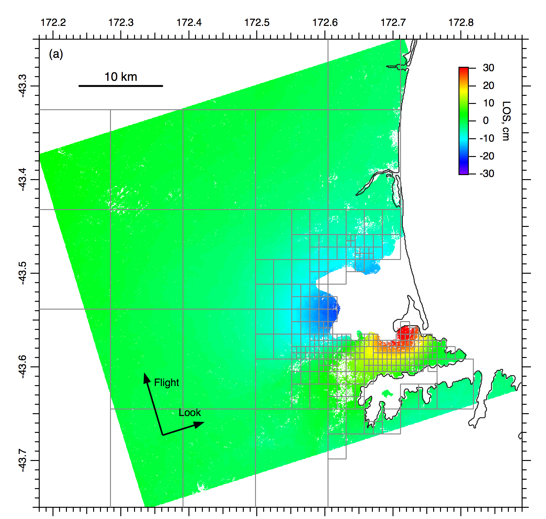
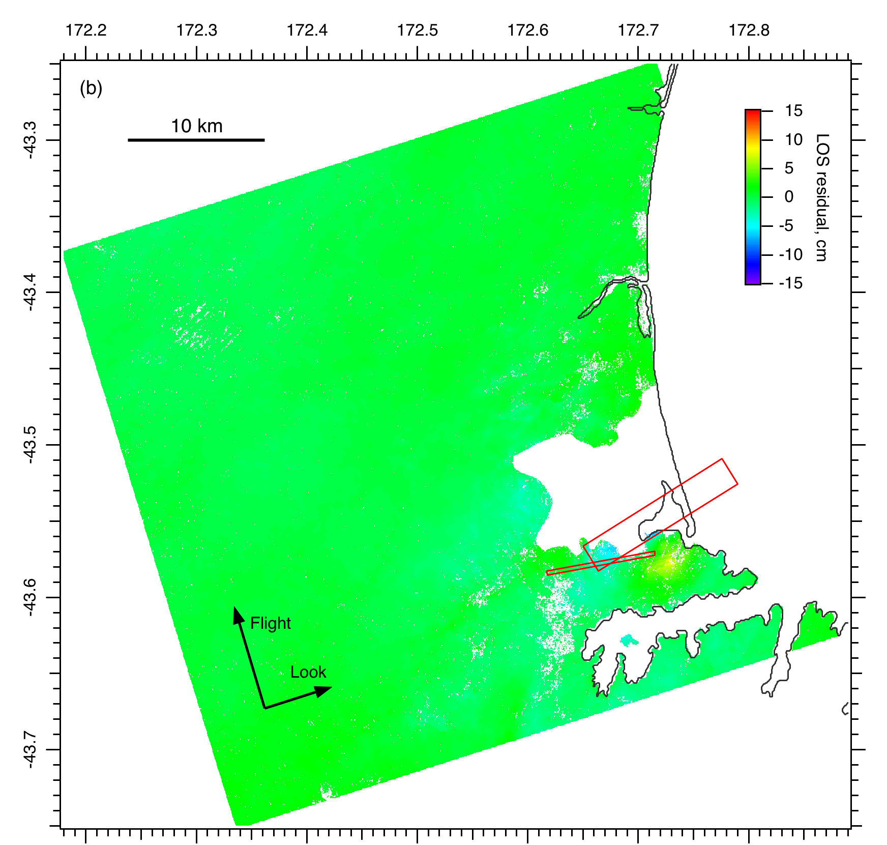
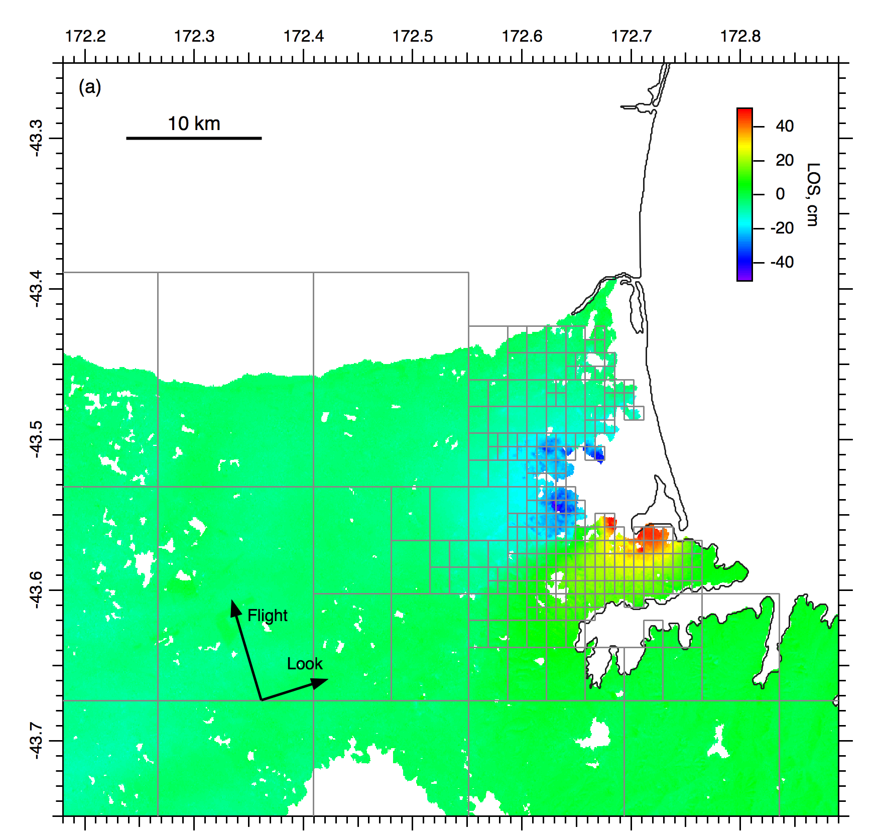
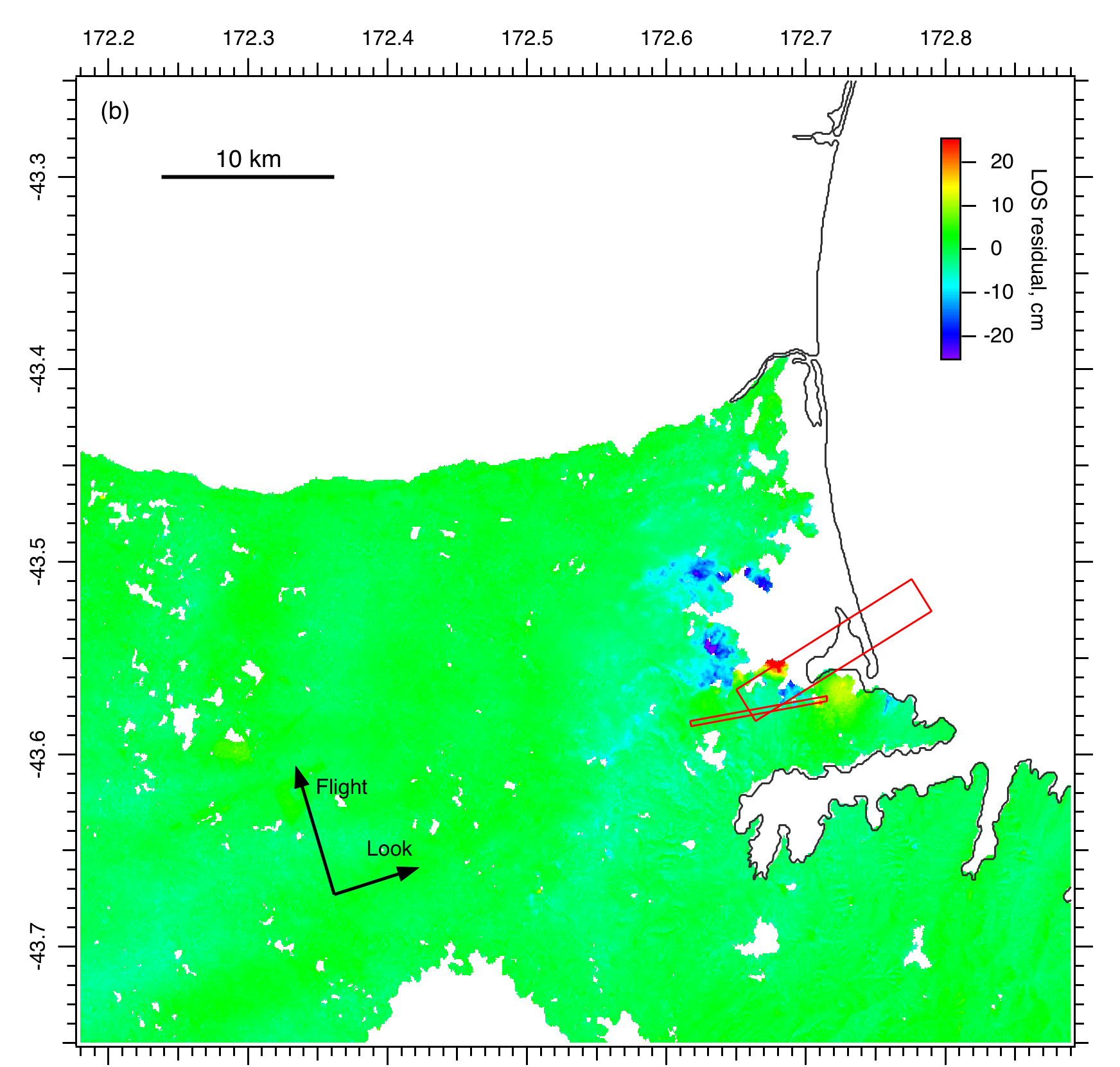
Figure S1. CSK ascending interferogram from 19 Feb - 23 Feb 2011. (a) Phase-unwrapped image; the grey boxes show the quadtree sampling of the image to provide data for the inversion. Red denotes ground displacement towards the satellite. (b) Residual after subtracting dislocation model fit and estimated linear orbital ramp, plotted at 2x scale; see Figure S4 for a version at larger scale. Red rectangles are the outlines of the model faults from Figure 6.
Figure S2. CSK descending interferogram from 20 Feb – 16 Mar 2011. (a) Phase-unwrapped image; the grey boxes show the quadtree sampling of the image to provide data for the inversion. Red denotes ground displacement towards the satellite. (b) Residual after subtracting dislocation model fit and estimated linear orbital ramp, plotted at 2x scale. Red rectangles are the outlines of the model faults from Figure 6.
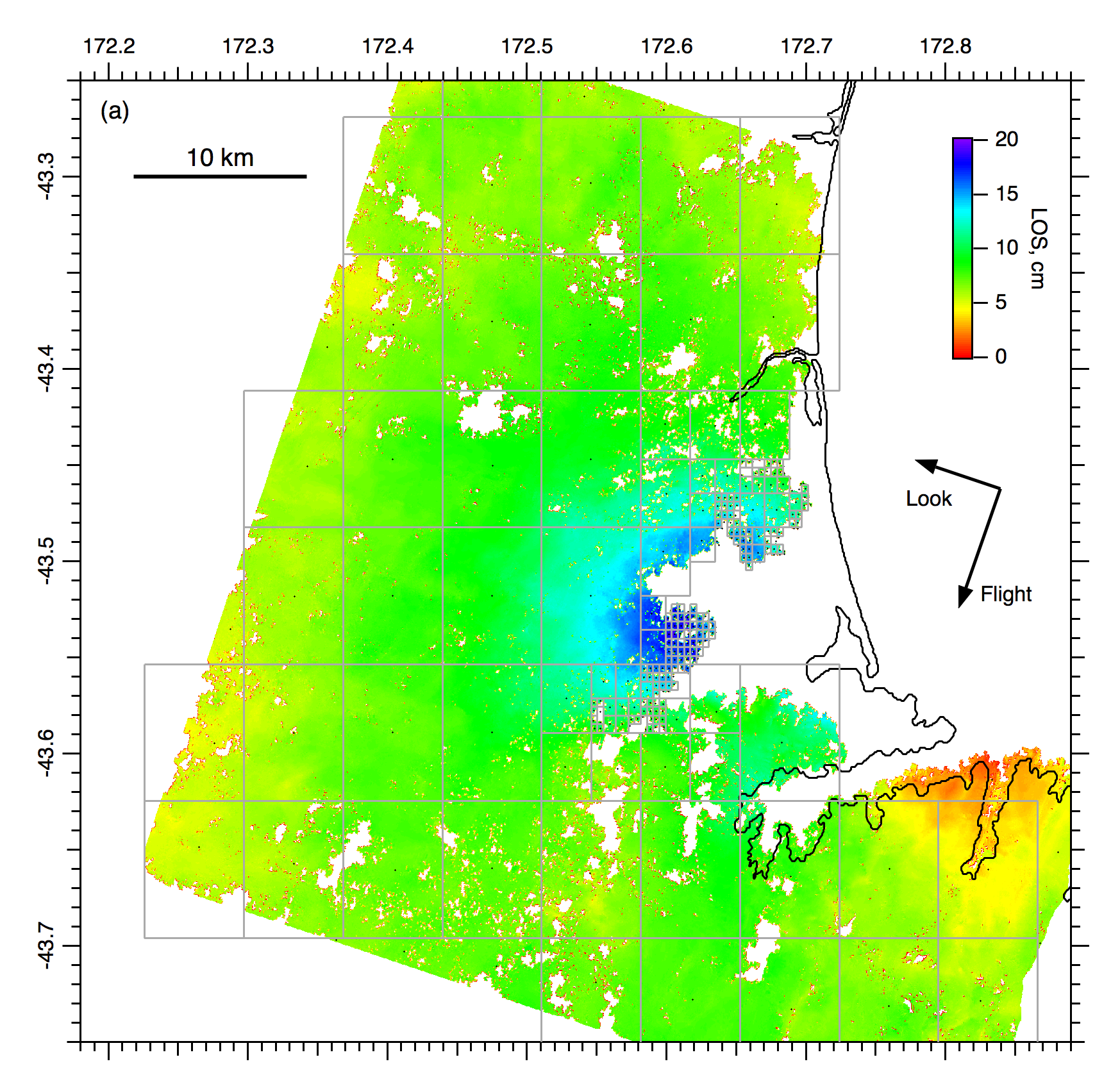
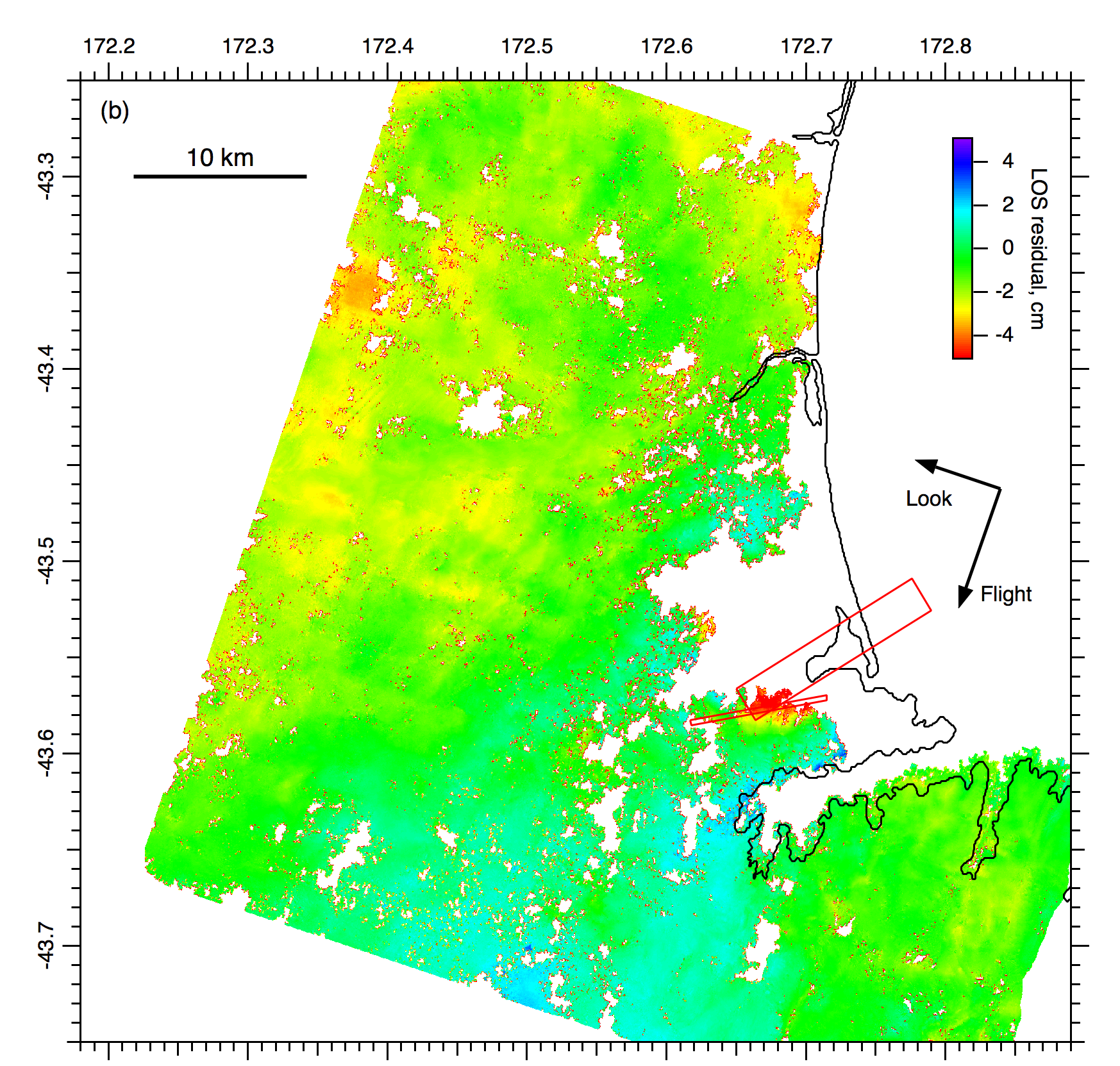
Figure S3. ALOS ascending interferogram from 27 Oct 2010 - 14 Mar 2011. (a) Phase-unwrapped image; the grey boxes show the quadtree sampling of the image to provide data for the inversion. Red denotes ground displacement towards the satellite. (b) Residual after subtracting dislocation model fit and estimated linear orbital ramp, plotted at 2x scale. Red rectangles are the outlines of the model faults from Figure 6.
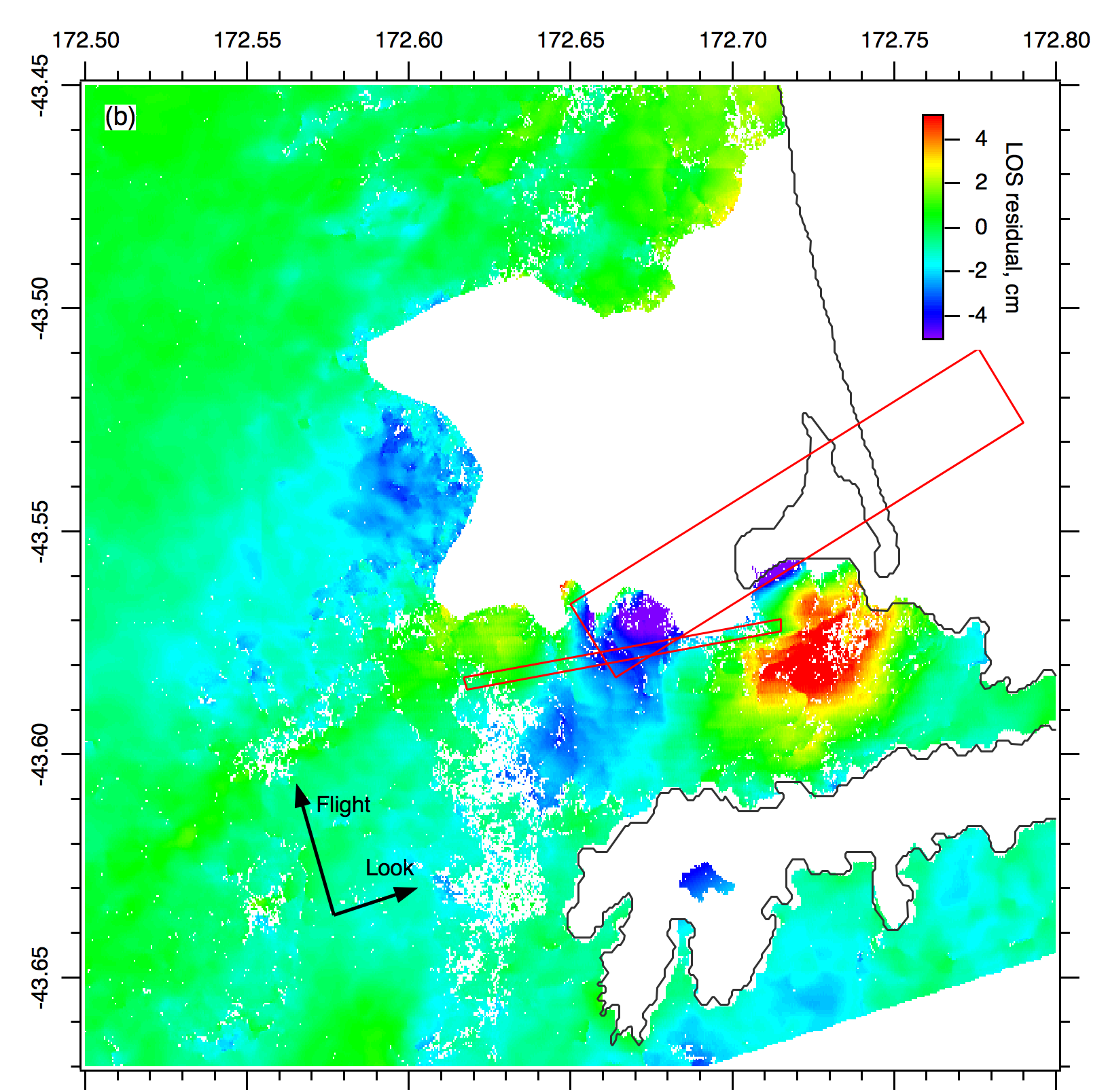
Figure S4. Expanded view of the central section of the CSK ascending residual from Figure S1b, in order to highlight that significant residuals remain in the near field.
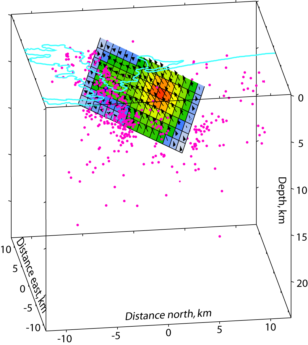
Figure S5. 3-D view from the east-southeast showing the location of the model fault of Figure 5, its slip distribution (hanging wall relative to footwall), and aftershocks (pink dots; mostly since February 22). The light blue line shows the coastline. Horizontal distances are measured from (43.55°S, 172.7°E).
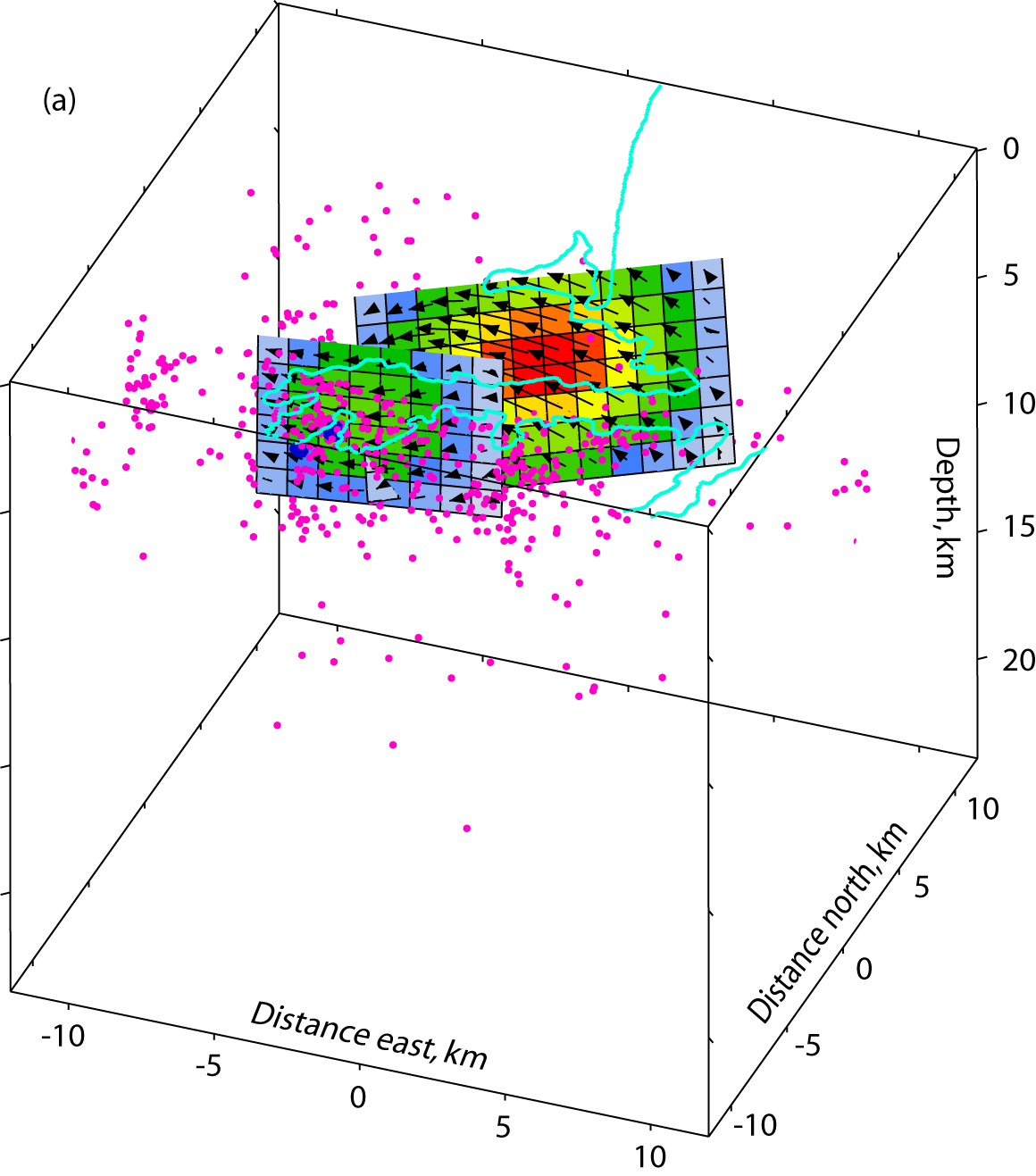
Figure S6a
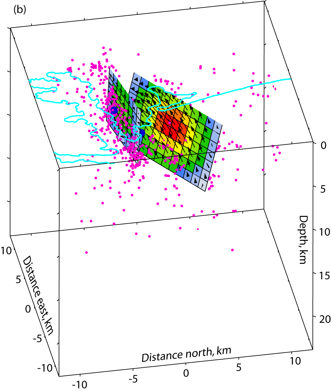
Figure S6b
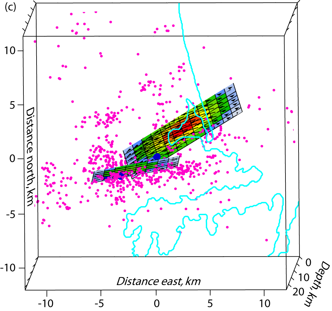
Figure S6c
Figure S6. 3-D views from (a) the south-southeast, (b) the east-southeast, and (c) above and south, showing the locations of the model faults of Figure 6, their slip distributions (hanging wall relative to footwall), and aftershocks (pink dots; mostly since February 22). The large blue dots are the hypocenters of the main shock and the two large aftershocks on February 22. The light blue line shows the coastline. There is a clear trend of small aftershocks nearly coincident with the fault plane inferred for the two large aftershocks. Horizontal distances are measured from (43.55°S, 172.7°E).
Table S1. Christchurch earthquake of 22 Feb 2011 (local time): GPS displacements and uncertainties in mm.
Table S2. Christchurch earthquake of 22 Feb 2011 (local time): Parameters of single-fault model corresponding to Figure 5 in main text.
Table S3. Christchurch earthquake of 22 Feb 2011 (local time): Parameters of two-fault model corresponding to Figure 6 in main text
[ Back ]