MoPaD is a newly developed software tool. It allows flexible visualisations of seimic sources by plotting focal sphere diagrams (FSDs), also known as "beachball representations".
Furthermore it provides decompositions of seismic moment tensors as well as transformations between the (strike, dip, slip-rake)-tuples and the moment tensor description of a source.
MoPaD is a command line tool!
In addition to a Python standard installation, the modules numpy and matplotlib are required. For using MoPaD, download the script named mopad and make it executable in your shell.
On this page you can find an alpha version of the source code of MoPaD, the license agreement, and some examples of usage and graphical outputs. For more information and the current version of the program visit http://www.mopad.org.
[ Up to Contents ]
The source code is written in Python; it contains basic Python classes and some additional script wrapping for using it from the standard shell. Therefore, all functionalities can be alternatively used by importing MoPaD as a Python module.
The version provided in this supplement is a functional alpha version (version 0.9 - 31.08.2011). It has been tested as a command line tool using Python versions 2.5 and 2.6 on Linux (Debian/Ubuntu) and on MacOS 10.
This is an alpha release version of the program MoPaD.
Use it only for testing purposes!
More recent user and developer versions are available upon request or from
http://www.mopad.org .
(Documentation and a short usage guide are available.)
MoPaD script:
(Alpha version 0.9 of MoPaD - only for testing - NO WARRANTY !! )
License:
(License agreement. Please keep it with the code!)
MoPaD is an open source program. It has been developed under the LGPL license. The license agreement should always be kept together with the code. Copyright by Lars Krieger and Sebastian Heimann 2010.
[ Up to Contents ]
mopad -h
mopad <method> -h
[ Up to Contents ]
Several visualisations of FSDs can be found in the publication. Here we provide the respective commands for generating most of those examples. The source mechanism is in all cases given by the seismic moment tensor M=(1,2,3,-4,-5,-10).
All example input lines given below directly generate files, which contain the respective plots. In order to obtain a visualisation window instead, just omit the -f option.
Filenames in parentheses denote files of plots, which are not explicitly generated by the stated commands. They are equivalent FSD visualisations but provided in various file formats.
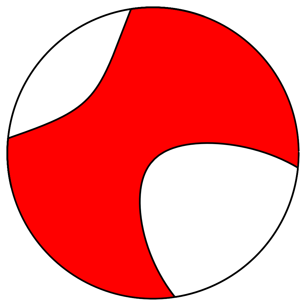
FSD_xmpl.png
( FSD_xmpl.ps )
( FSD_xmpl.pdf )
( FSD_xmpl.svg )
( FSD_xmpl.eps )
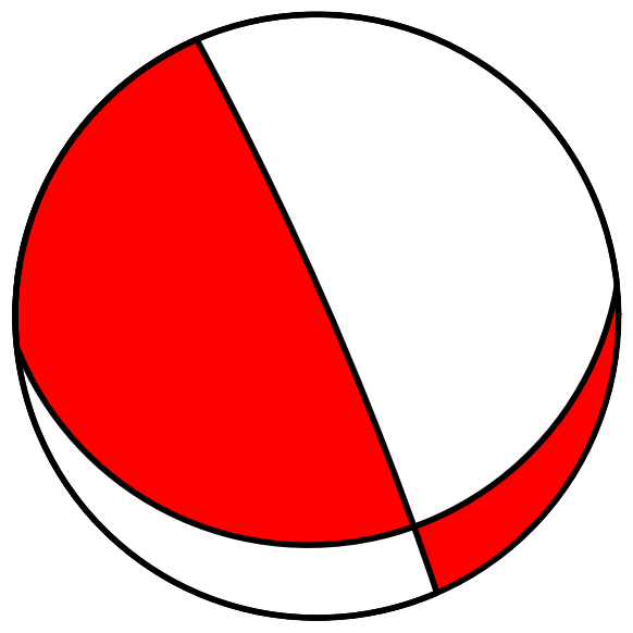
A standard graphical
representation of the FSD: stereographic back-hemisphere projection in vertical view,
North is situated at the upper edge, pressure area in white, tension
area in red, isotropic component is included.
Generated using the command
mopad plot 1,2,3,-4,-5,-10 -I -f FSD_xmpl.png
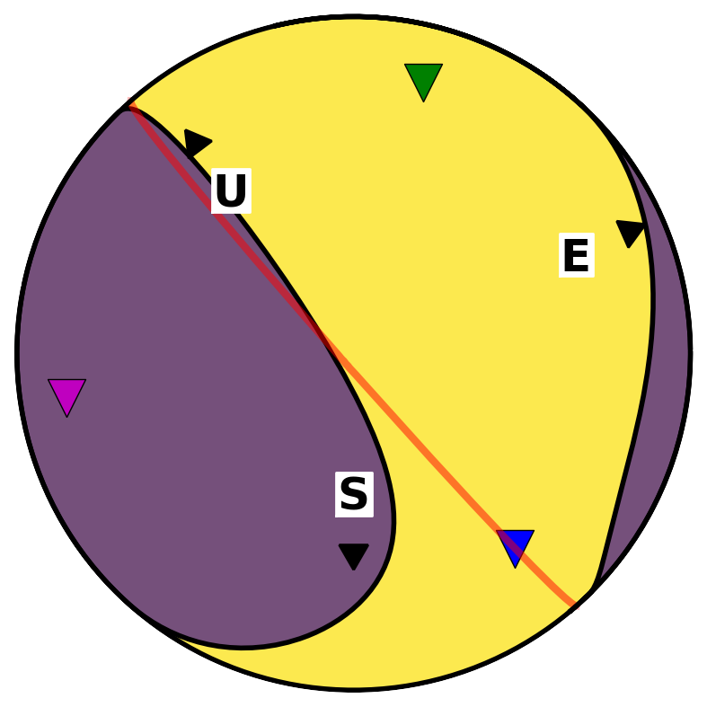
FSD_complex.svg
( FSD_complex.png )
A highly unusal visualisation of the FSD, including the following features:
- Output-size 10 cm
- Reduced to the deviatoric part
- View from South-East
- Showing the front hemisphere
- Using orthographic projection
- Tensional domain in yellow
- Pressure domain in purple
- Showing in red the fault plane '1' of the governing double couple part
- Indication of the positions of the eigenvectors
- Annotated axes of the basis system
Generated using the command
mopad plot 1,2,3,-4,-5,-10 -s 10 -v -50,30,-0 -U
      -p o -f FSD_complex.svg -r 252,233,79 -w 117,80,123
      -d 1 3 red 0.5 -e 15 4 1 -b
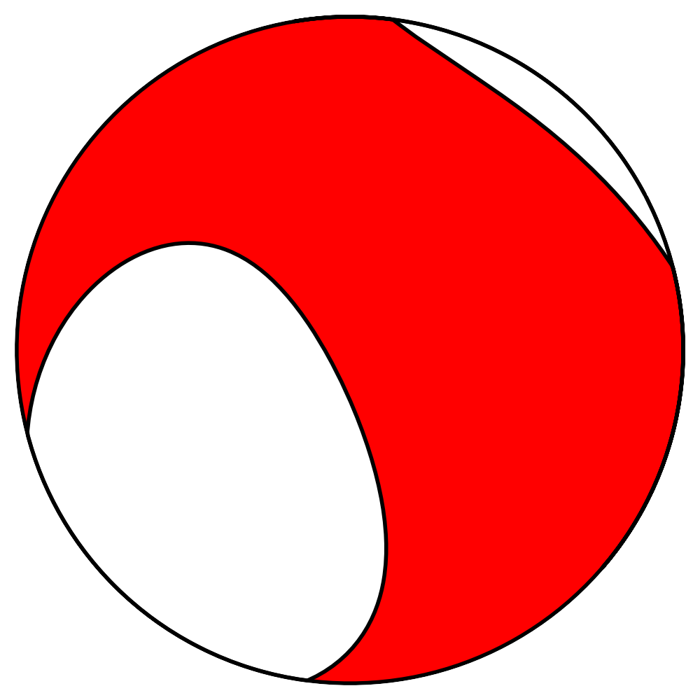
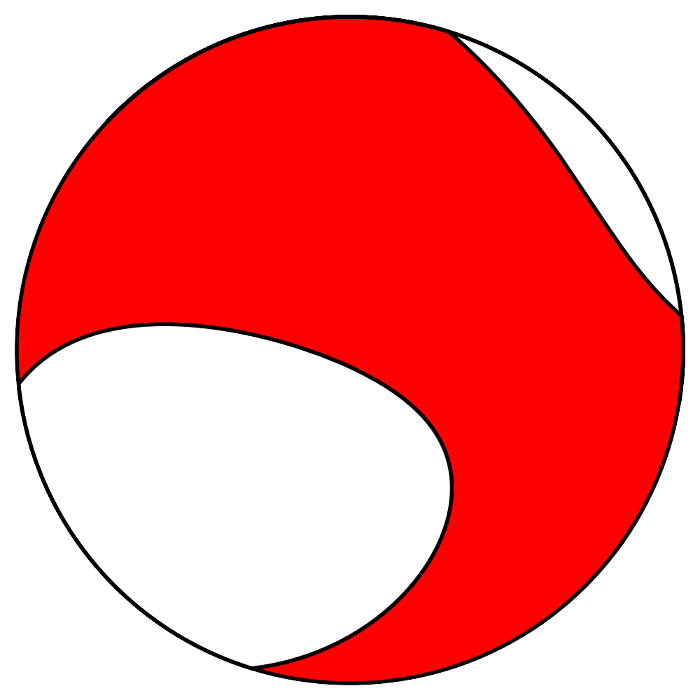
FSD_xmpl_upper.svg
( FSD_xmpl_upper.png )
Plot of the front-projection (upper hemisphere) of the FSD.
Generated using the command
mopad plot 1,2,3,-4,-5,-10 -I -U -f FSD_xmpl_upper.svg
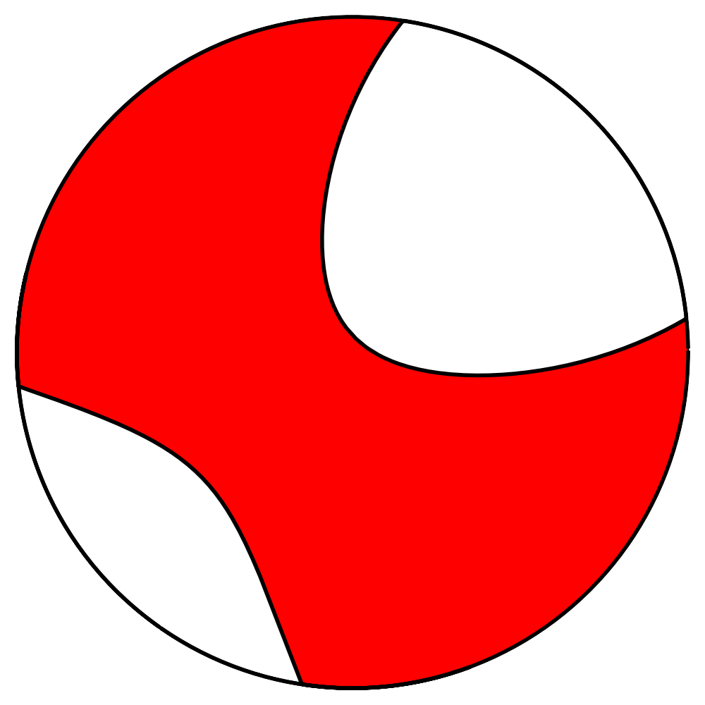
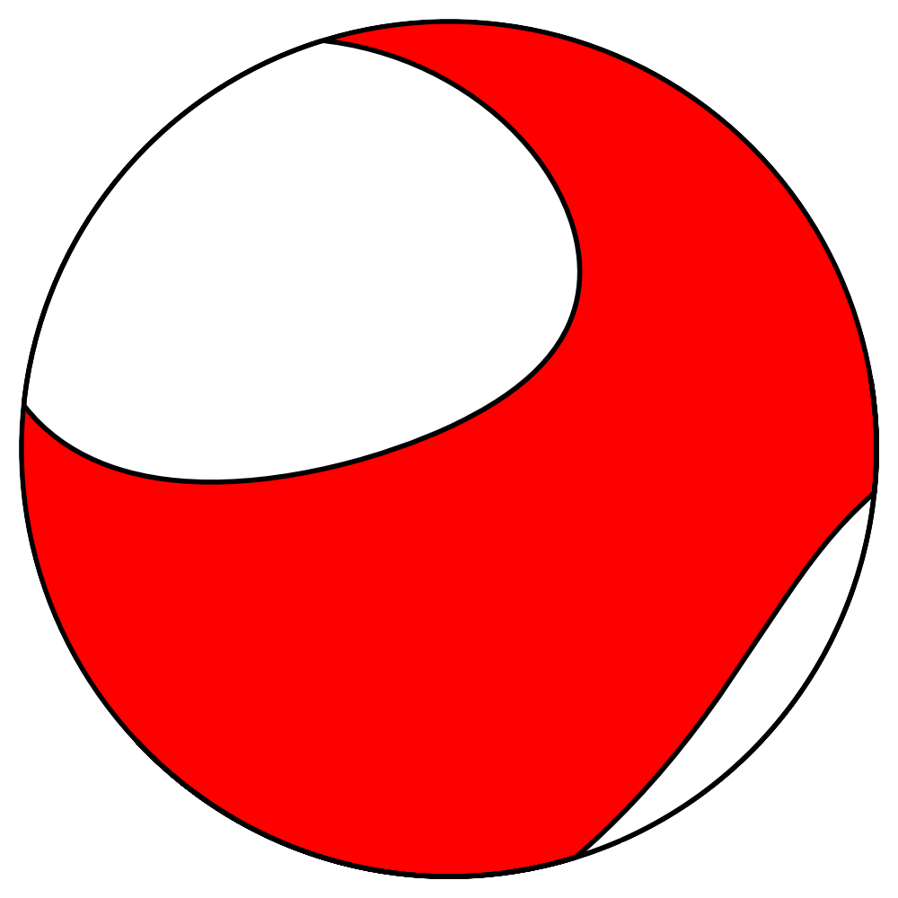
FSD_xmpl_north.png
FSD_xmpl_east.png
FSD_xmpl_south.png
FSD_xmpl_west.png
Plots of the back-projections for 4 vertical cross sections of the FSD,
as seen from North, East, South, West.
Generated using the commands
mopad plot 1,2,3,-4,-5,-10 -I -v 90,0,180 -f FSD_xmpl_north.png
mopad plot 1,2,3,-4,-5,-10 -I -v 0,90,90 -f FSD_xmpl_east.png
mopad plot 1,2,3,-4,-5,-10 -I -v -90,0,0 -f FSD_xmpl_south.png
mopad plot 1,2,3,-4,-5,-10 -I -v 0,-90,-90 -f FSD_xmpl_west.png
FSD_xmpl_full.png
FSD_xmpl_iso.png
FSD_xmpl_devi.png
FSD_xmpl_dc.png
FSD_xmpl_clvd.png
Plots of vertical back-projection FSDs for various parts of M:
- Full moment tensor
- Isotropic part
- Deviatoric part
- Double couple component
- CLVD component
Generated using the commands
mopad plot 1,2,3,-4,-5,-10 -I -s 1 -f FSD_xmpl_full.png
mopad plot 1,2,3,-4,-5,-10 -P iso -s 0.36 -f FSD_xmpl_iso.png
mopad plot 1,2,3,-4,-5,-10 -s 0.93 -f FSD_xmpl_devi.png
mopad plot 1,2,3,-4,-5,-10 -P dc -s 0.74 -f FSD_xmpl_dc.png
mopad plot 1,2,3,-4,-5,-10 -P clvd -s 0.57 -f FSD_xmpl_clvd.png
(Sizes are square roots of percentage in order to obtain linearity in area.)
[ Up to Contents ]
Obtain an overview over all important parameters of the source mechanism (provided here as 6 matrix entries of M in the USE convention) by using the command
mopad describe 1,2,3,-4,-5,-10 -i USE
yielding
Scalar Moment: M0 = 14.9031 Nm (Mw = -5.3)
Moment Tensor: Mnn =  0.200,  Mee =  0.300, Mdd =  0.100,
               Mne =  1.000,  Mnd = -0.400, Med =  0.500    [ x 10 ]


Fault plane 1: strike =  95°, dip =  67°, slip-rake = -163°
Fault plane 2: strike = 358°, dip =  74°, slip-rake =  -24°
The source mechanism can also be provided as a tuple of angles (strike, dip, slip-rake; given in degrees). Optionally, the scalar seismic moment can be provided as a fourth input value:
mopad describe 30,60,-45,7e15
yielding
Scalar Moment: M0 = 7e+15 Nm (Mw = 4.5)
Moment Tensor: Mnn = -0.264,  Mee =  0.693, Mdd = -0.429,
               Mne =  0.029,  Mnd = -0.338, Med =  0.091    [ x 1e+16 ]


Fault plane 1: strike =  30°, dip =  60°, slip-rake =  -45°
Fault plane 2: strike = 147°, dip =  52°, slip-rake = -141°
[ Up to Contents ]
MoPaD can help to plot non-standard FSDs in GMT
generated maps. The gmt method of MoPaD returns a
string of (x,y)-values, which can be used as input for psxy.
Output values are given in Euklidian (rectangular) coordinates centered at (0,0). According to the projection used in GMT, these must be externally transformed to the appropriate coordinate system.
psxy_fill.cpt
A colour table which defines the colour of the filling of the tensional area (psxy color code '1') and the pressure area (psxy color code '0') of the focal sphere. In this example it is red (1) and white (0).
This example table has been generated with the GMT command
makecpt -Cpolar -Z
psxy_lines.cpt
A colour table which defines the colour of the nodal and border lines (psxy color code '1') of the FSD. In this example it is black (1).
This example table has been generated with the GMT command
makecpt -I -Chot -Z
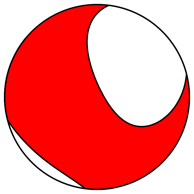
BB1.ps
A *.ps-file containing the 'standard' FSD for M=(1,2,3,-4,-5,-10),
generated with MoPaD, plotted with GMT.
Generated with MoPaD's gmt command in combination with psxy:
mopad gmt 1,2,3,-4,-5,-10 -t fill -p s | psxy -Jx4/4 -R-2/2/-2/2 -P
  -Cpsxy_fill.cpt -M -K -L  > BB1.ps && mopad gmt 1,2,3,-4,-5,-10 -t
  lines -p s | psxy -Jx4/4 -R-2/2/-2/2 -W5 -P -Cpsxy_lines.cpt -M
  -O >> BB1.ps
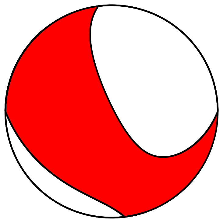
BB2.ps
A *.ps-file containing the FSD for the same M, but with a rotated view
and using an orthographic projection. The new viewpoint is defined by
(latitude=45, longitude=45, local counter clockwise rotation of the
view=45)
Generated with MoPaD's gmt command in combination with psxy:
mopad gmt 1,2,3,-4,-5,-10 -t fill -p o -v 45,45,45 | psxy -Jx4/4
  -R-2/2/-2/2 -P -Cpsxy_fill.cpt -M -K -L > BB2.ps && mopad gmt
  1,2,3,-4,-5,-10 -t lines -p o -v 45,45,45 | psxy -Jx4/4 -R-2/2/-2/2 -W5
  -P -Cpsxy_lines.cpt -M -O >> BB2.ps
[ Up to Contents ]
Obtain a full standard decomposition in USE basis of the source mechanism (provided as 6 matrix entries in the NED convention) by using the command
mopad decompose 1,2,3,-4,-5,-10 -o USE
yielding
 Basis system of the input:

NED

 Basis system of the output:

USE

 Decomposition type:

ISO + DC + CLVD

 Full moment tensor in USE-coordinates:

  /  0.30 -0.50  1.00 \
  | -0.50  0.10  0.40  |   x  10.000000
  \  1.00  0.40  0.20 /


 Isotropic part in USE-coordinates:

  /  2.00  0.00  0.00 \
  |  0.00  2.00  0.00  |
  \  0.00  0.00  2.00 /


 Isotropic percentage:

13

 Deviatoric part in USE-coordinates:

  /  0.10 -0.50  1.00 \
  | -0.50 -0.10  0.40  |   x  10.000000
  \  1.00  0.40  0.00 /


 Deviatoric part in USE-coordinates:

  /  0.10 -0.50  1.00 \
  | -0.50 -0.10  0.40  |   x  10.000000
  \  1.00  0.40  0.00 /


 Deviatoric percentage:

87

 Double Couple part in USE-coordinates:

  /  1.36 -2.97  7.30 \
  | -2.97 -1.77  1.95  |
  \  7.30  1.95  0.41 /


 Double Couple percentage:

55

 Second Double Couple part in USE-coordinates:

 not available in this decomposition type


 Second Double Couple's percentage:

 not available in this decomposition type


 Third Double Couple part in USE-coordinates:

 not available in this decomposition type


 Third Double Couple's percentage:

 not available in this decomposition type


 CLVD part in USE-coordinates:

  / -0.36 -2.03  2.70 \
  | -2.03  0.77  2.05  |
  \  2.70  2.05 -0.41 /


 CLVD percentage:

32

 Seismic moment (in Nm) :

14.9031089939

 Moment magnitude Mw:

-5.25114874821

 Eigenvalues T N P :

12.5907, 4.31243, -10.9031

 Eigenvectors T N P (in basis system USE):

  / -0.74 \
  |  0.09  |
  \ -0.67 /

  /  0.26 \
  | -0.88  |
  \ -0.40 /

  / -0.62 \
  | -0.47  |
  \  0.63 /


 Tension-axis in USE -coordinates:

  / -0.62 \
  | -0.47  |
  \  0.63 /


 Null-axis in USE -coordinates:

  /  0.26 \
  | -0.88  |
  \ -0.40 /


 Pressure-axis in USE -coordinates:

  / -0.74 \
  |  0.09  |
  \ -0.67 /
[ Up to Contents ]
[ Back ]