Electronic Supplement to
Rapid Estimation of Fault Parameters for Tsunami Warning along the Mexican Subduction Zone: A Scenario Earthquake in the Guerrero Seismic Gap

doi: 10.1785/0220120156

by Xyoli Pérez-Campos, Diego Melgar, Shri K. Singh, Víctor Cruz-Atienza, Arturo Iglesias, Vala Hjörleifsdóttir

This Electronic Supplement contains the figures in color for emphasis and the links for the synthetic data generated by Cruz-Atienza et al. (2011) of the M_w8.2 Guerrero-gap rupture scenario used in this study.

Figures

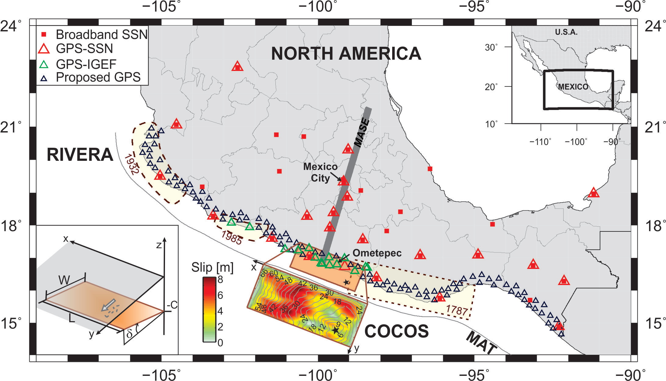
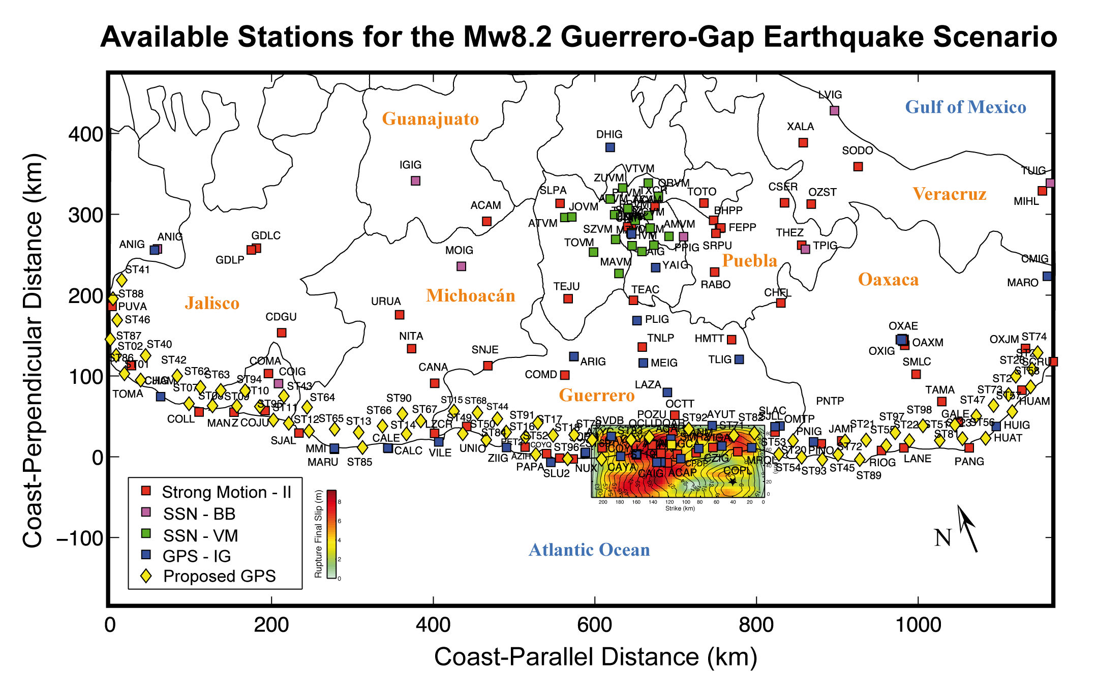
▲ Figure S1. Guerrero rupture scenario, broadband seismic network and GPS station locations. Rupture areas for historic earthquakes (M ≥ 8) are denoted by the elongated dashed shapes. The rupture area for the 1787, the 1932, and the 1985 earthquakes are taken from Suárez and Albini (2009), Singh et al. (1985), and UNAM Seismology Group (1986), respectively. The location of the MASE profile is shown as a thick gray line. The rupture area used by Cruz-Atienza et al. (2011) for the scenario earthquake is shown as an orange rectangle, slip on the fault is in meters and rupture time contours in seconds, the black star denotes the epicenter. MAT = Middle America Trench. SSN = Servicio Sismológico Nacional; GPS-SSN = GPS network operated by the SSN, with real-time transmission capacity of 1 sample per second; GPS-IGEF = autonomous GPS stations operated by individual researchers or groups from the Instituto de Geofísica, UNAM. Geometry from Okada (1992) is in the lower corner: L and W are the length and the width of the fault, respectively, δ is the dip and –C is the depth of the downdip edge of the fault. x and y axes are oriented along and perpendicular to the coast (towards to the trench), respectively. For coastal GPS stations y ≈ 0.

---

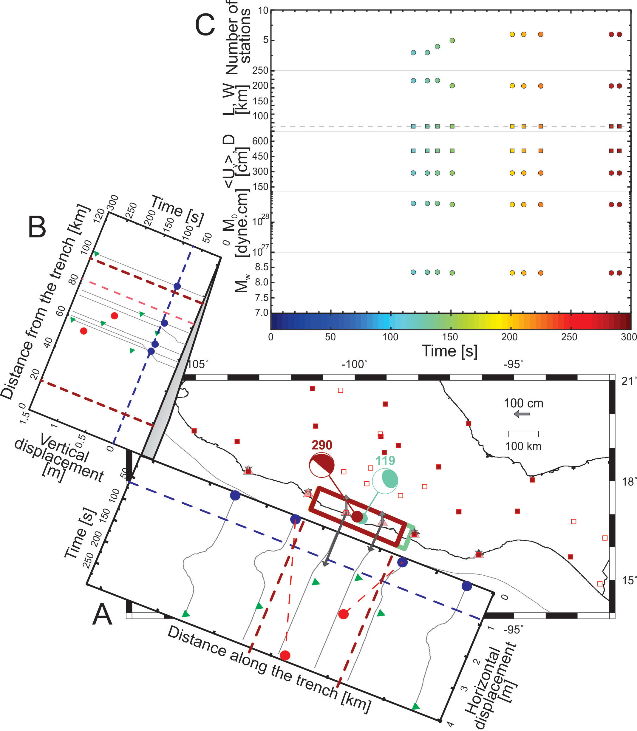
▲ Figure S2. Results from test 1. Fault parameters from GPS-SSN stations with real-time transmission capability and focal mechanism from W-phase inversion using regional broadband stations. Map shows the GPS stations as triangles, solid symbols for those that detected the event within 3 minutes. The broadband stations are denoted by squares and stations used in the W-phase inversion by solid symbols. Displacement vectors are shown for each station, dark gray for U_y (displacement perpendicular to the trench) and light gray for U_z (vertical displacement). Solid circles on the map, show the location of the epicenter used for the W-phase inversion (center of the fault), the color corresponds to time: 119 s in green and 290 s in red. The focal mechanisms show the results from the W-phase inversion at 119 s (green) and 290 s (red). A: Moving average of U_y with respect to time, and with distance along the trench. Triangles show the time when the static coseismic displacement is determined for each station. Solid circles represent the value of U_y ≥ (U_y)₂₀ in blue, and U_y < (U_y)₂₀ in red. The dash blue line denotes U_y = (U_y)₂₀. Thin dashed red lines denote de linear regression used to find the intercept with U_y = (U_y)₂₀ to establish the fault lateral limits, denoted by the thick red dashed lines. B: Moving average of U_z with respect to time and with distance from the trench. Triangles show the time when the static coseismic displacement is determined for each station. Solid circles represent the value of U_y, U_y ≥ (U_y)₂₀ in blue, and U_y < (U_y)₂₀ in red. The dash blue line denotes U_z = 0. Thin dashed red line denote the change from U_z > 0 to U_z < 0; the updip and downdip limits are denoted by the thick red dashed lines. C: Solutions with time. Each column of symbols corresponds to the solution obtained at that time. For the second row, circles correspond to L and squares to W, W_s is denoted by the dashed line. For the third row, circles correspond to <U_y> and squares to D.

---

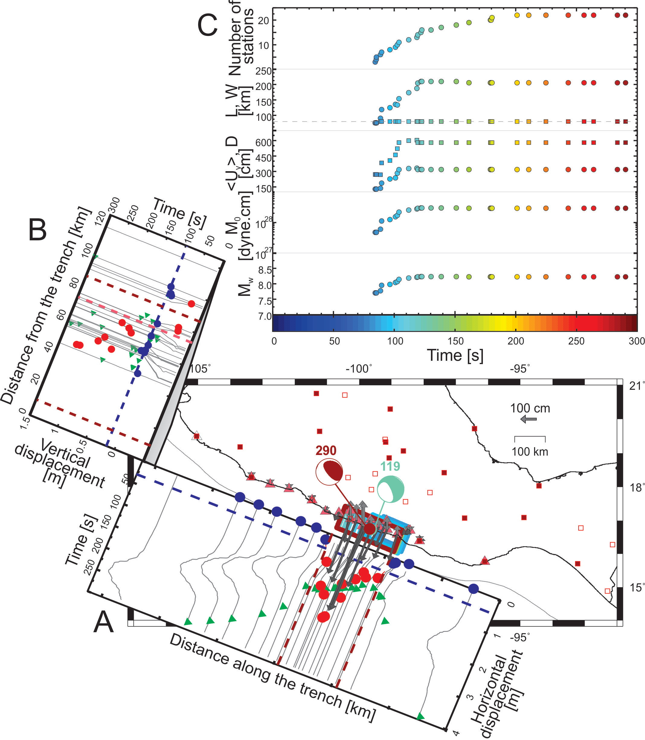
▲ Figure S3. Results from test 2. Fault parameters from existing 22 GPS stations along the coast and focal mechanism from W-phase inversion using regional broadband stations. Symbols and panels are the same as for figure 2.

---

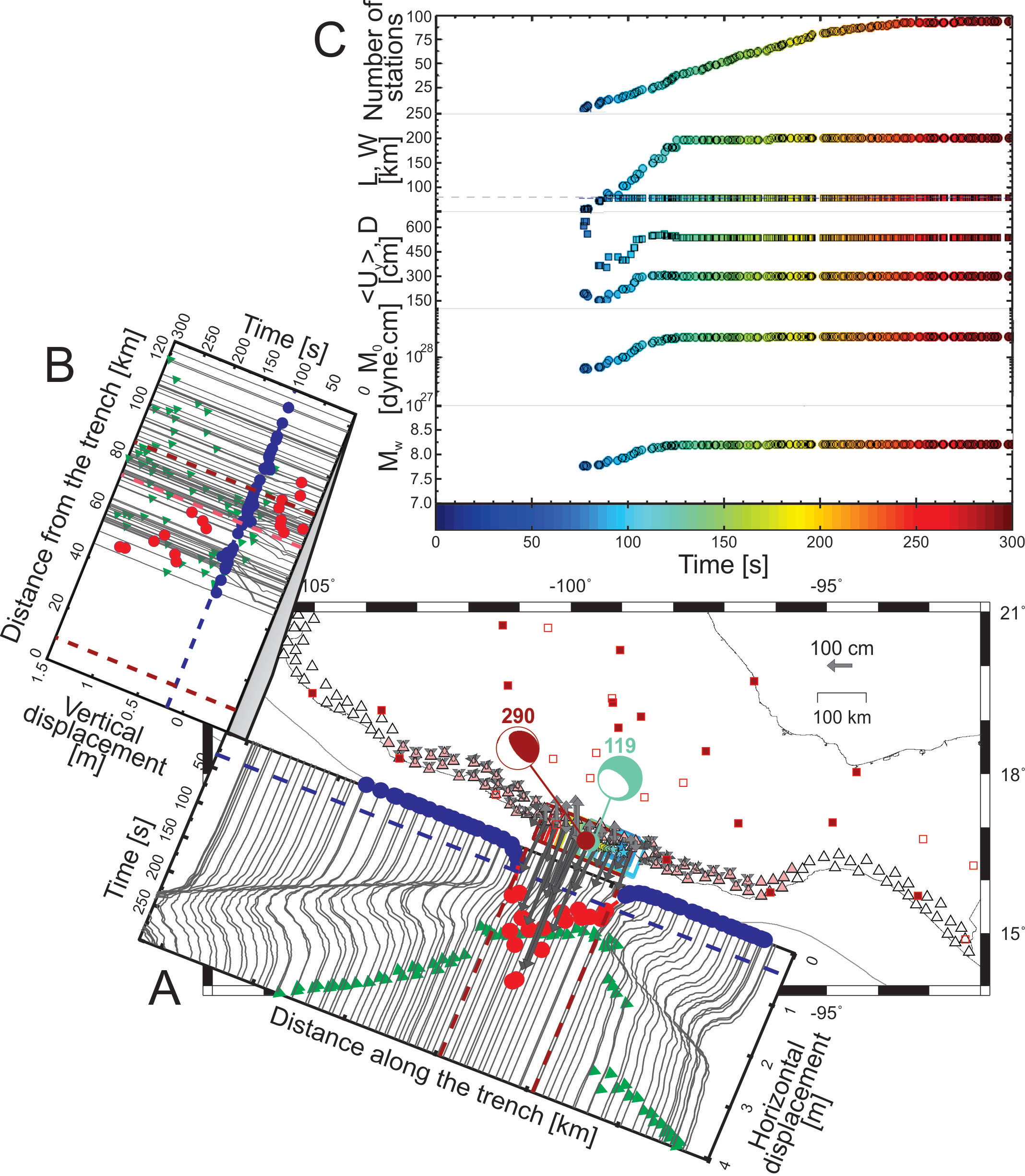
▲ Figure S4. Results from test 3. Fault parameters from proposed GPS station configuration along the coast and focal mechanism from W-phase inversion using regional broadband stations. Symbols and panels are the same as for figure 2.

---

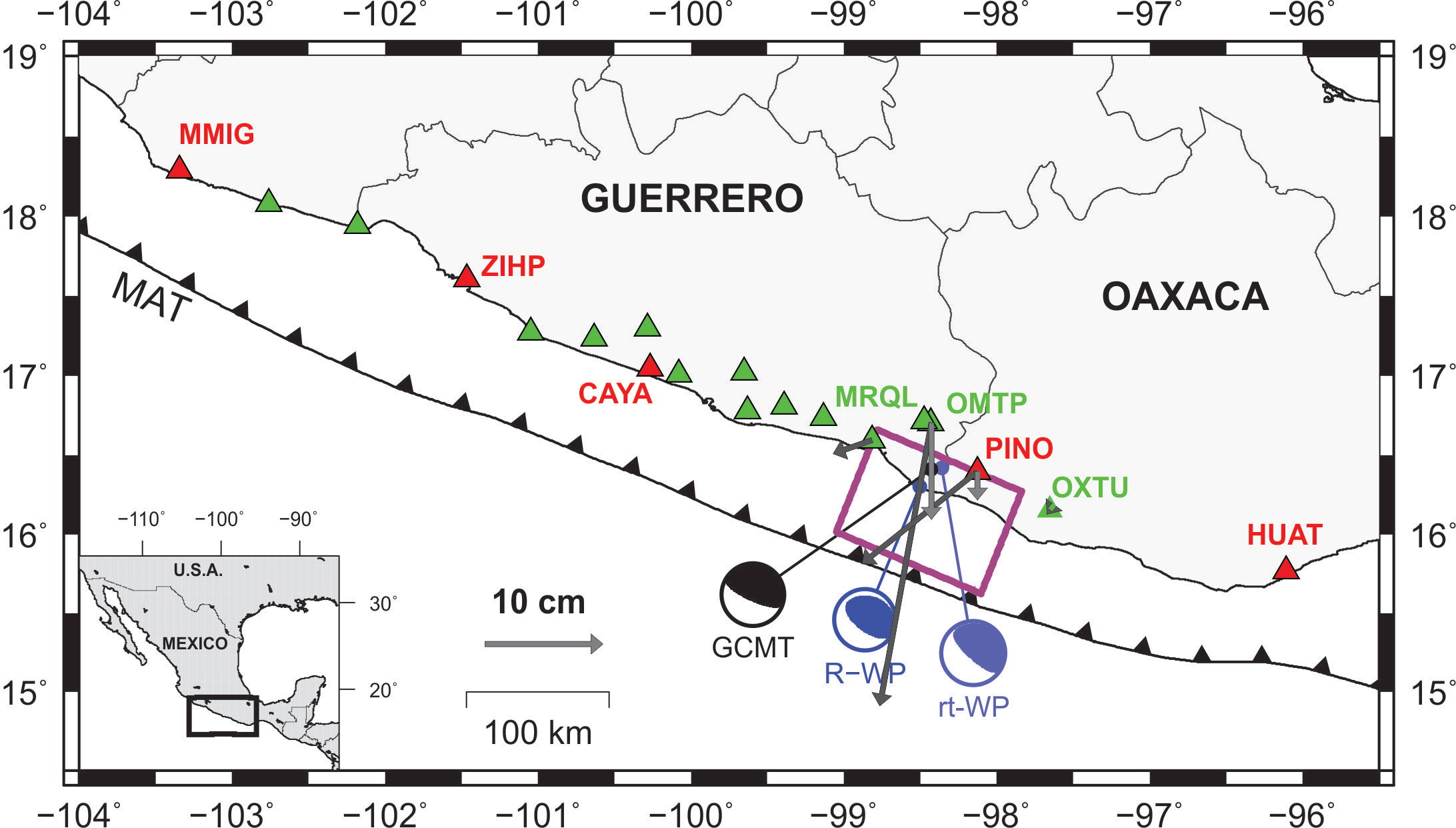
▲ Figure S5. Fault parameters for the 20 March 2012 Ometepec earthquake (M_w7.4). Triangles denote GPS stations: GPS-SSN in red, GPS-IGEF in green. Rectangle corresponds to the fault solution. Focal mechanism in light blue corresponds to the real-time solution from W-phase inversion (rt-WP), reported by the SSN; in blue is the revised W-phase inversion (R-WP); in black is the solution reported by Global CMT (GCMT, http://www.globalcmt.org).

---

Synthetic Data

Data generated by Cruz-Atienza et al. (2011) of the M_w8.2 Guerrero-gap rupture scenario. Besides the displacement records in the GPS networks used in this study, namely the UNAM 'Instituto de Geofísica' (I de G) (www.geofisica.unam.mx)network and the one proposed here, we also provide all the available data for this scenario including both velocity seismograms in the broadband stations of the 'Servicio Sismológico Nacional' (SSN) (http://www.ssn.unam.mx) and acceleration seismograms at the free-field strong-motion stations of the UNAM 'Instituto de Ingeniería' (I de I) (http://www.iingen.unam.mx).

Stations Map for the Scenario Earthquake
Proposed GPS Network	Displacement Seismograms [Zip Archived ASCII; ~3.7 MB]	Stations Coordinates [ASCII; 4 KB]
I de G GPS Network	Displacement Seismograms [Zip Archived ASCII; ~1.6 MB]	Stations Coordinates [ASCII; 4 KB]
SSN Broadband Network	Velocity Seismograms [Zip Archived ASCII; ~2.3 MB]	Stations Coordinates [ASCII; 4 KB]
I de I Strong Motion Network	Acceleration Seismograms [Zip Archived ASCII; ~5 MB]	Stations Coordinates [ASCII; 4 KB]

All seismograms are lowpass filtered at 0.8 Hz, which corresponds to the numerical-accuracy upper limit, and are given in the international metric system [mks] with time increment of 0.12 s.

---

[ Back ]

References

Cruz-Atienza, V. M., V. Hjörleifsdóttir, and A. Rocher (2011). Simulando un Mw8.2 en la brecha de Guerrero, Reunión Anual 2011, Unión Geofísica Mexicana, Geos, 31, 150.
Okada, Y. (1992). Internal deformation due to shear and tensile faults in a half space, Bull. Seismol. Soc. Am., 82, 1018–1040.
Singh, S. K., G. Suarez, and T. Dominguez (1985). The Oaxaca, Mexico earthquake of 1931: Lithospheric normal faulting in the subducted Cocos plate, Nature, 137, 56–58.
Suárez, G., and P. Albini (2009). Evidence for great tsunamigenic earthquakes (M 8.6) along the Mexican subduction zone, Bull. Seismol. Soc. Am., 99, 892–896.
UNAM Seismology Group (1986). The September 1985 Michoacan earthquakes: Aftershock distribution and history of rupture, Geophys. Res. Lett., 13, 573–576.