Electronic Supplement
to
ObsPyLoad - a tool for fully automated retrieval of seismological
waveform data
by Chris Scheingraber, Kasra Hosseini, Robert Barsch, and Karin Sigloch
This Electronic Supplement contains an exemplary waveform summary plot, several diagrams, the full output of the long help function, as well as the source file of the script along with installation instructions.
A. Supplementary Figures
Figure S1. Options and schematic program flow
A diagram of the program flow and the most important options.
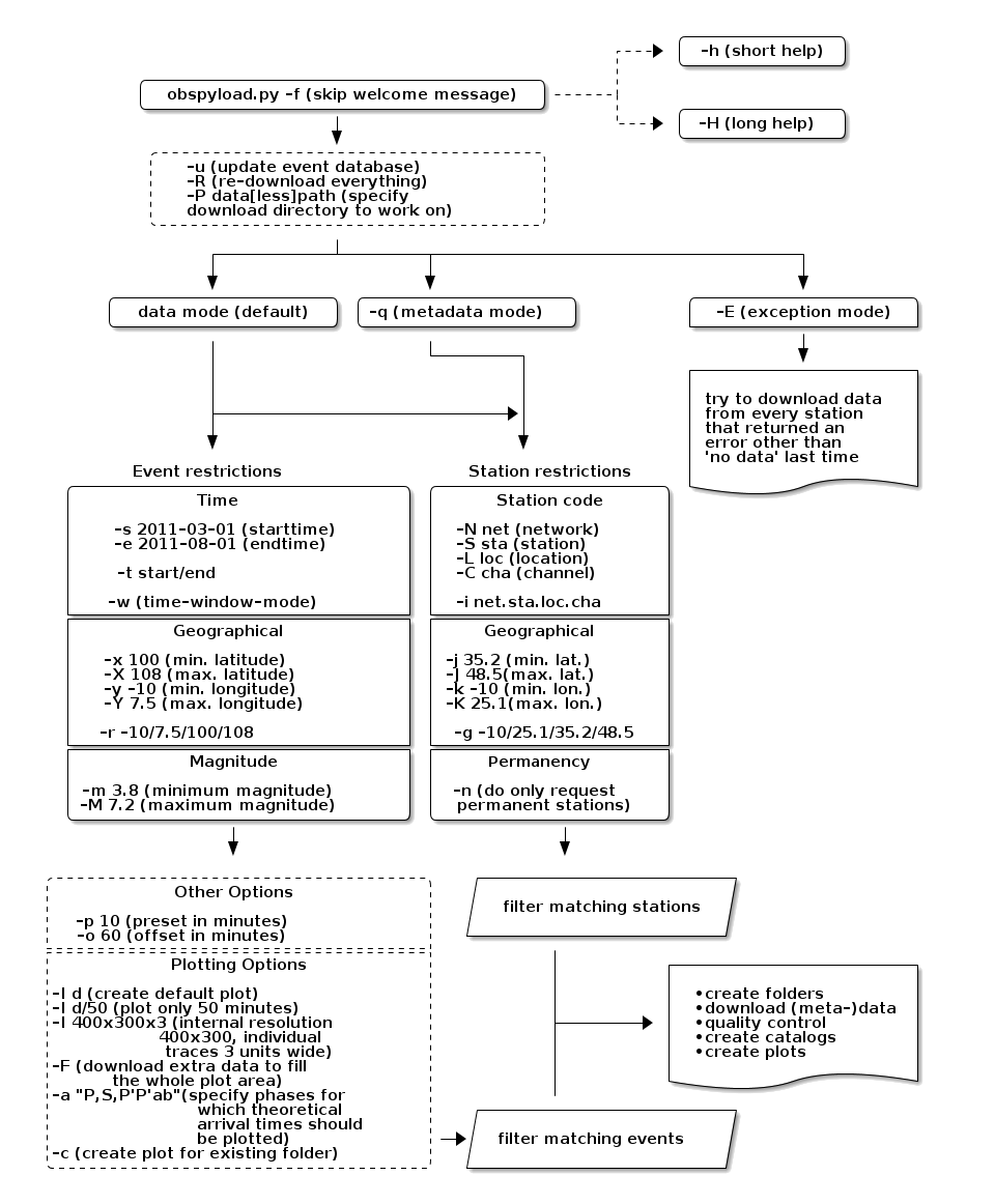
Figure S2. Folder structure in data download mode
A diagram of the directory structure as it is generated automatically for each event-based call to ObsPyLoad. The default name of the top-level directory, obspyload-data, may be overridden by the -P option, e.g. -P tohoku events. For each matching event, a subfolder is generated, into which the corresponding seismograms and metadata are sorted.
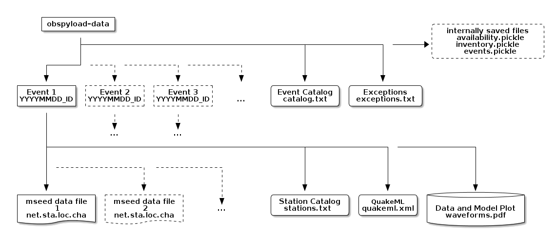
Figure S3. Folder structure in metadata download mode
This is the folder structure generated when the script is instructed to download metadata.
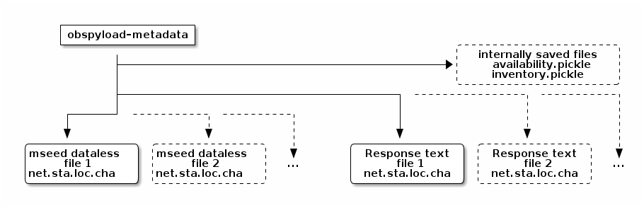
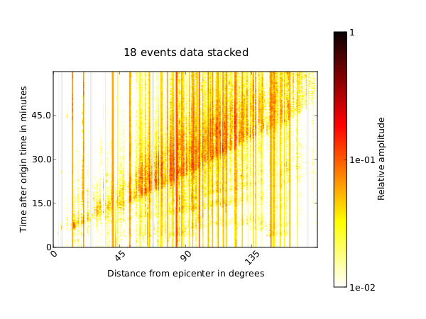
Figure S4. Alternative waveform summary plot
A waveform plot as automatically generated by ObsPyLoad. Each vertical line represents one or more seismograms. This is an alternative version that avoids data-free time windows (-F option). 18 M_w > 7.7 events stacked, no theoretical arrival times overlain (-a none option), vertical component data. The actual plots are saved as PDF files.
B. Source code and dependencies
The ObsPyLoad waveform retrieval tool as described in the paper
may be downloaded here. The newest version is available at the
ObsPy repository.
For all functionality, ObsPyLoad depends on the ObsPy framework for
processing seismological data.
Download: obspyload.py [Plain Text Python Script, version as described in the paper; 131 KB].
The newest version of this script can be downloaded from the ObsPy
repository:
https://raw.github.com/obspy/branches/master/scheingraber/obspyload.py
The required ObsPy seismological framework can be downloaded from:
http://www.obspy.org.
C. Installation and system requirements
C.1 Installing ObsPy on GNU/Linux
For the Debian and Ubuntu distributions, an ObsPy apt repository is maintained. To add the repository to your system, append it to the file /etc/apt/sources.list (as root):
deb http://deb.obspy.org squeeze main
Replace squeeze with the codename of your Debian/Ubuntu release. Currently supported releases are lenny and squeeze for Debian, and lucid, maverick, natty and oneiric for Ubuntu.
To import the ObsPy gnupg key so that apt is able to check the integrity of the downloaded packages, the following commands need to be executed once (as root):
wget
http://obspy.org/export/2889/obspy/trunk/misc/debian/public.key
apt-key add public.key
To install ObsPy with dependencies, run once (as root):
apt-get update
apt-get install python-obspy
If you are not using Debian or Ubuntu (or some close enough derivative), visit the ObsPy website at http://www.obspy.org/ for a detailed description of the installation procedure.
C.2 Installing ObsPy on Mac OSX
The fastest way to obtain a working Python and ObsPy environment
under OSX is the ObsPy OSX Application. Due to the great work of
the ObsPy team, the installation is as easy as dragging the
ObsPy.app icon to the OSX Applications folder. You can obtain the
ObsPy OSX Application from:
https://github.com/obspy/obspy/wiki/Installation-on-Mac-with-OSX-Application.
C.3 Installing ObsPy on Microsoft Windows
For installation on Windows, the convenient ObsPy Installer
which will automatically download and install all requirements, can be downloaded from:
https://github.com/obspy/obspy/wiki/Installation-on-Windows.
C.4 Installing ObsPyLoad
Once a working Python and ObsPy environment is installed, download the newest version of ObsPyLoad from https://raw.github.com/obspy/branches/master/scheingraber/obspyload.py (or use the version as described in the paper, see A).
Normally, ObsPyLoad uses the default Python interpreter of the system. If necessary, the first line (shebang) of the script can be changed to specify another Python interpreter. For instance, many OSX users might want use the Python environment from the ObsPy OSX Application. To achieve this, it is sufficient to change the first line of obspyload.py to:
#!/Applications/ObsPy.app/Contents/MacOS/bin/python
To be used as illustrated in the examples in the paper, the script has to be moved to any directory contained in the path (i.e. /usr/local/bin/).
D. Output of the long help function
The output of the long help function may be generated with obspyload.py --more-help:


ObsPyLoad: ObsPy Seismic Data Download tool.
============================================


There are two different flavors of usage, in short:
===================================================

  e.g.:            obspyload.py -r <lonmin>/<lonmax>/<latmin>/<latmax>-t
                   <start>/<end> -m <min_mag> -M <max_mag> -i <net.sta.loc.cha>
  e.g.:            obspyload.py -y <min_lon> -Y <max_lon> -x <min_lat> -X
                   <max_lat> -s <start> -e <end> -P <datapath> -o <offset>
                   --reset -f


You may provide (no mandatory options):
=======================================

SOURCE (event) restrictions:
----------------------------

* specify a timeframe:

  Default:         the last 1 month
  Format:          Any obspy.core.UTCDateTime recognizable string.

  -t[--time]       <start>/<end>
                   e.g.: -t 2007-12-31/2011-01-31

  -s[--start]      <starttime>
  -e[--end]        <endtime>
                   e.g.: -s 2007-12-31 -e 2011-01-31


* specify a minimum and maximum magnitude:

  Default:         minimum magnitude 5.8, no maximum magnitude.
  Format:          Integer or decimal.

  -m[--magmin]     <min.magnitude>
  -M[--magmax]     <max.magnitude>
                   e.g.: -m 4.2 -M 9


* specify rectangular geographical source region:

  Default:         no constraints.
  Format:          +/- 90 decimal degrees for latitudinal limits,
                   +/- 180 decimal degrees for longitudinal limits.

  -r[--rect]       <min.longitude>/<max.longitude>/<min.latitude>/<max.latitude>
                   e.g.: -r -15.5/40/30.8/50

  -x[--lonmin]     <min.longitude>
  -X[--lonmax]     <max.longitude>
  -y[--latmin]     <min.latitude>
  -Y[--latmax]     <max.latitude>
                   e.g.: -x -15.5 -X 40 -y 30.8 -Y 50


RECEIVER (station) restrictions:
--------------------------------

* specify rectangular geographical receiver region:

  Default:         no constraints.
  Format:          +/- 90 decimal degrees for latitudinal limits,
                   +/- 180 decimal degrees for longitudinal limits.

  -g[--station-    <min.longitude>/<max.longitude>/<min.latitude>/<max.latitude>
  rect]
                   e.g.: -g -15.5/40/30.8/50

  -k[--sta-        <min.latitude>
  lonmin]
  -K[--sta-        <max.longitude>
  lonmax]
  -j[--sta-        <min.latitude>
  latmin]
  -J[--sta-        <max.latitude>
  latmax]
                   e.g.: -k -15.5 -K 40 -j 30.8 -J 50


* specify circular geographical receiver region:

  Default:         no constraints.
  Format:          +/- 90 decimal degrees for latitudinal center,
                   +/- 180 decimal degrees for longitudinal center,
                   from 0 to 180 decimal degrees for radius.

  -l[--sta-        <longitude>/<latitude>/<max.radius>
  radius]
                   e.g.: -l 11/48/20


* specify a station identifier restriction:

  Default:         no constraints.
  Format:          Any station code, may include wildcards.

  -i[--identity]   <nw>.<st>.<l>.<ch>
                   e.g. -i IU.ANMO.00.BH* or -i *.*.?0.BHZ

  -N[--network]    <network>
  -S[--station]    <station>
  -L[--location]   <location>
  -C[--channel]    <channel>
                   e.g. -N IU -S ANMO -L 00 -C BH*

* additional station options:

  -n[--no-
  temporary]
                   Instead of downloading both temporary and permanent networks
                   (default), download only permanent ones.

  -p[--preset]     <preset>
                   Time parameter given in seconds which determines how close
                   the data will be cropped before estimated arrival time at
                   each individual station. Default: 5 minutes.

  -o[--offset]     <offset>
                   Time parameter given in seconds which determines how close
                   the data will be cropped after estimated arrival time at each
                   individual station. Default: 40 minutes.

  -q[--query-
  resp]
                   Instead of downloading seismic data, download instrument
                   response files.


PLOTTING options:
-----------------

  Default:         no plot. If the plot will be created with -I d (or -I
                   default), the defaults are 1200x800x1/100 and the default
                   phases to plot are 'P' and 'S'.

  -I[--plot]       <pxHeight>x<pxWidth>x<colWidth>[/<timespan>]
                   For each event, create one plot with the data from all
                   stations together with theoretical arrival times. You may
                   provide the internal plotting resolution: e.g. -I 900x600x5.
                   This gives you a resolution of 900x600, and 5 units broad
                   station columns. If -I d, or -I default, the default of
                   1200x800x1 will be used. If this command line parameter is
                   not passed to ObsPyLoad at all, no plots will be created. You
                   may additionally specify the timespan of the plot after event
                   origin time in minutes: e.g. for timespan lasting 30 minutes:
                   -I 1200x800x1/30 (or -I d/30). The default timespan is 100
                   minutes. The final output file will be in pdf format.

  -F[--fill-
  plot]
                   When creating the plot, download all the data needed to fill
                   the rectangular area of the plot. Note: depending on your
                   options, this will approximately double the data download
                   volume (but you'll end up with nicer plots ;-)).

  -a[--phases]     <phase1>,<phase2>,...
                   Specify phases for which the theoretical arrival times should
                   be plotted on top if creating the data plot(see above, -I
                   option). Default: -a P,S. To plot all available phases, use
                   -a all. If you just want to plot the data and no phases, use
                   -a none.
                   Available phases:
                   P, P'P'ab, P'P'bc, P'P'df, PKKPab, PKKPbc, PKKPdf, PKKSab,
                   PKKSbc, PKKSdf, PKPab, PKPbc, PKPdf, PKPdiff, PKSab, PKSbc,
                   PKSdf, PKiKP, PP, PS, PcP, PcS, Pdiff, Pn, PnPn, PnS, S,
                   S'S'ac, S'S'df, SKKPab, SKKPbc, SKKPdf, SKKSac, SKKSdf,
                   SKPab, SKPbc, SKPdf, SKSac, SKSdf, SKiKP, SP, SPg, SPn, SS,
                   ScP, ScS, Sdiff, Sn, SnSn, pP, pPKPab, pPKPbc, pPKPdf,
                   pPKPdiff, pPKiKP, pPdiff, pPn, pS, pSKSac, pSKSdf, pSdiff,
                   sP, sPKPab, sPKPbc, sPKPdf, sPKPdiff, sPKiKP, sPb, sPdiff,
                   sPg, sPn, sS, sSKSac, sSKSdf, sSdiff, sSn
                   Note: if you select phases with ticks(') in the phase name,
                   don't forget to use quotes (-a "phase1',phase2") to avoid
                   unintended behaviour.

  -c[--create-
  plots]
                   Create plots for an existing data folder previously
                   downloaded without the plotting option. May be used with -P
                   to specify the path and with -a to specify the phases. Has to
                   be used together with -I to specify the plot properties.


FOLDER Options:
---------------

  -P[--datapath]   <datapath>
                   Specify a different datapath, do not use do default one.

  -R[--reset]
                   If the datapath is found, do not resume previous downloads as
                   is the default behaviour, but redownload everything. Same as
                   deleting the datapath before running ObsPyLoad.

  -u[--update]
                   Update an existing folder, adding new events and newly
                   available data for existing events.

  -f[--force]
                   Skip working directory warning (auto-confirm folder
                   creation).

Type obspyload.py -h for a list of all long and short options.


Examples:
---------

(1) Alps region, minimum magnitude of 4.2:

    obspyload.py -r 5/16.5/45.75/48 -m 4.2
                 --start 2007-01-13T08:24:00 --end 2011-02-25T22:41:00


(2) Sumatra region, Christmas 2004, different timestring, mind the quotation marks:

    obspyload.py -r 90/108/-7/7 -t "2004-12-24 01:23:45/2004-12-26 12:34:56" -m 9


(3) Mount Hochstaufen area(Ger/Aus), default minimum magnitude:

    obspyload.py -r 12.8/12.9/47.72/47.77 -t 2001-01-01/2011-02-28


(4) Only one station, to quickly try out the plot:

    obspyload.py -s 2011-03-01 -m 9 -I 400x300x3 -f -i IU.YSS.*.*


(5) ArcLink Network wildcard search:

    obspyload.py -N B? -S FURT -f


(6) Downloading metadata from all available stations to folder "metacatalog":

    obspyload.py -q -f -P metacatalog

(7) Download stations that failed last time:

    obspyload.py -E -P thisOrderHadExceptions -f


(8) Add plots to an existing folder 'myfolder' specifying some plotting options:

    obspyload.py -c -P myfolder -I 1200x800x5/60 -a P,S,PP
E. Usage as a Python module
In addition to previously described stand-alone functionality, it is also possible to import ObsPyLoad as a module within another Python script. The function parameters are analogous to the command line.
from obspyload import main as opl
opl(start="2011-02-27", end="2011-04-16", magmin=7.0, lonmin=140,
lonmax=146, latmin=30, latmax=42, lo=00, ch=BHZ,
plt="1200x800x5/60", datapath="tohoku_events", force=True)
Note that these are the same options as for the first example in the quick tour. To access the documentation in a Python shell, you may invoke:
help(opl)
[ Back ]