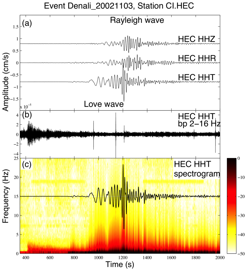
Figure S1. The 3-component broadband seismograms (a), 2-16 Hz band-pass-filtered transverse component (b), and the corresponding spectrogram (d) recorded by the station CI.HEC and generated by the 2002 Denali Fault earthquake. Other symbols and notations are the same as Figure 2.
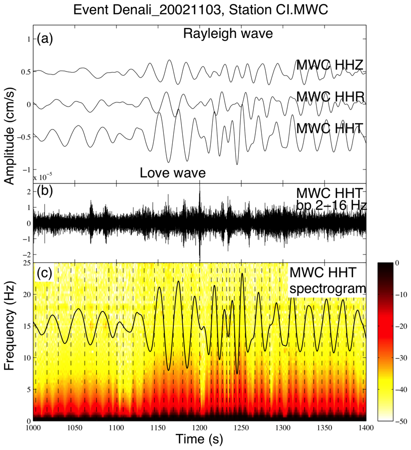
Figure S2. A zoom-in plot of Figure 2 around the large-amplitude surface waves showing that the high-frequency energy in the spectrogram (c) is mostly associated with the zero crossings (vertical dashed lines) in the transverse-component seismogram.
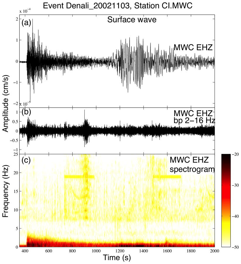
Figure S3. (a) Vertical-component raw seismograms generated by the 2002 Mw7.8 Denali Fault earthquake and recorded at the short-period station CI.MWC in Southern California. (b) 2-16 Hz band-pass-filtered transverse-component seismogram showing locally generated high-frequency signals. (c) The spectrogram of the transverse-component seismogram at station CI.MWC. Other symbols and notations are the same as Figure 2.
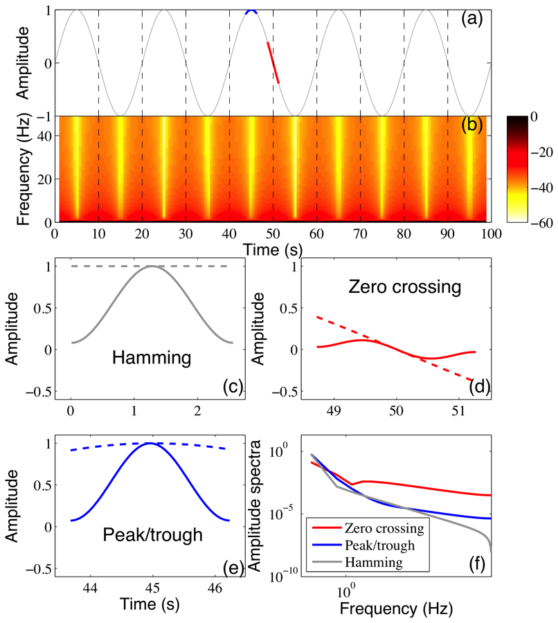
Figure S4. (a) A sine function with a period of 20 s. A Hamming window is applied to the segments marked with red (zero crossing) and blue (peak/trough) respectively. The resulting time series after the Hamming window are shown in (d) and (e), and the corresponding spectra are shown in (f). The vertical dashed lines mark the zero crossing. (b) The spectrogram computed using the “spectrogram” command in Matlab. The corresponding input parameters are given in the main text. (c) The Hamming window (solid) and data with amplitude = 1 (dashed). (d) The truncated data around zero crossing (dashed) and after applying the Hamming window (solid). (e) The truncated data around the peak/trough (dashed) and after applying the Hamming window (solid). (f) The Fourier spectra of the Hamming window (light gray), the windowed zero crossing (red), and windowed peak/trough (blue).
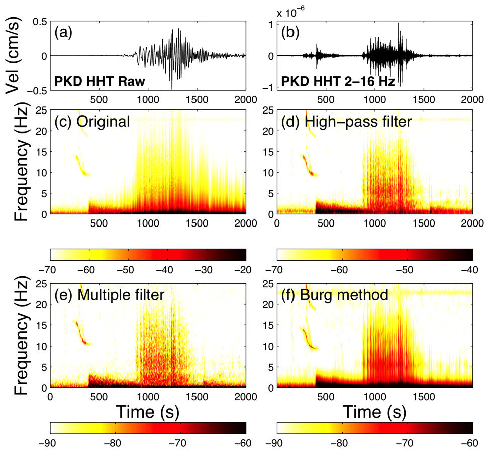
Figure S5. A comparison of the spectrogram for the transverse-component data at BK.PKD with and without corrections. Other symbols and notations are the same as in Figure 5.
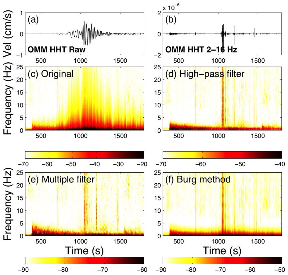
Figure S6. A comparison of the spectrogram for the transverse-component data at NN.OMM with and without corrections. Other symbols and notations are the same as in Figure 5.
[ Back ]