This electronic supplement contains results and related material for mass–transceiver combinations other than the three detailed in the main article (i.e., for mass–transducer combinations D–K in Table 1 of the main article and Figs. S1 and S2), drawings and photographs of liquid proof masses, amplitude and phase transfer functions (TFFs), clip and linearity tests, and noise plots. Combinations A–C and their performance are described in the main article; here, we include the graphical results from A to C for reference and comparison to the D–K combinations of mass and transducer.
A (LQ.RP.P.H2O) is described in the main article.
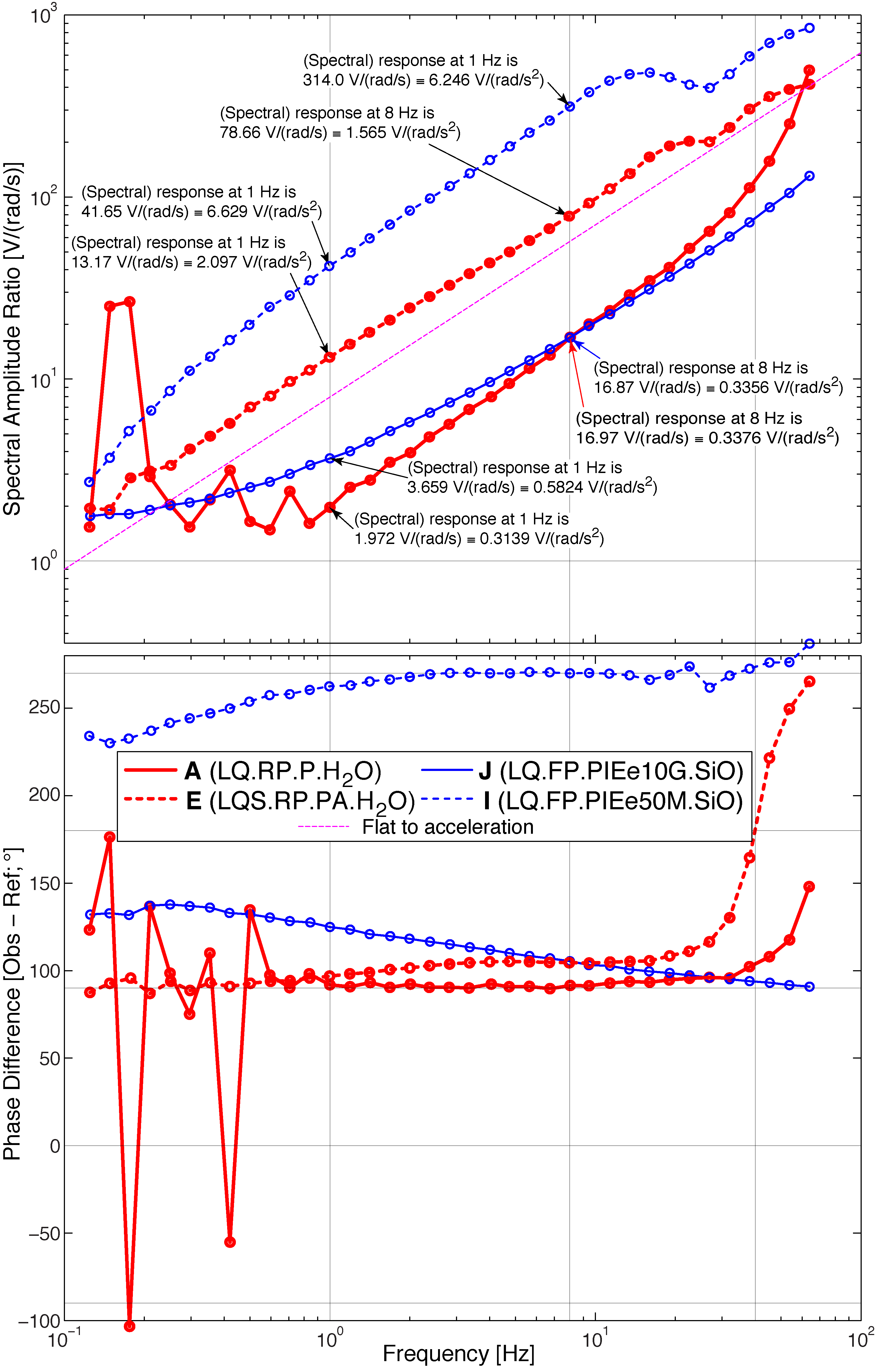
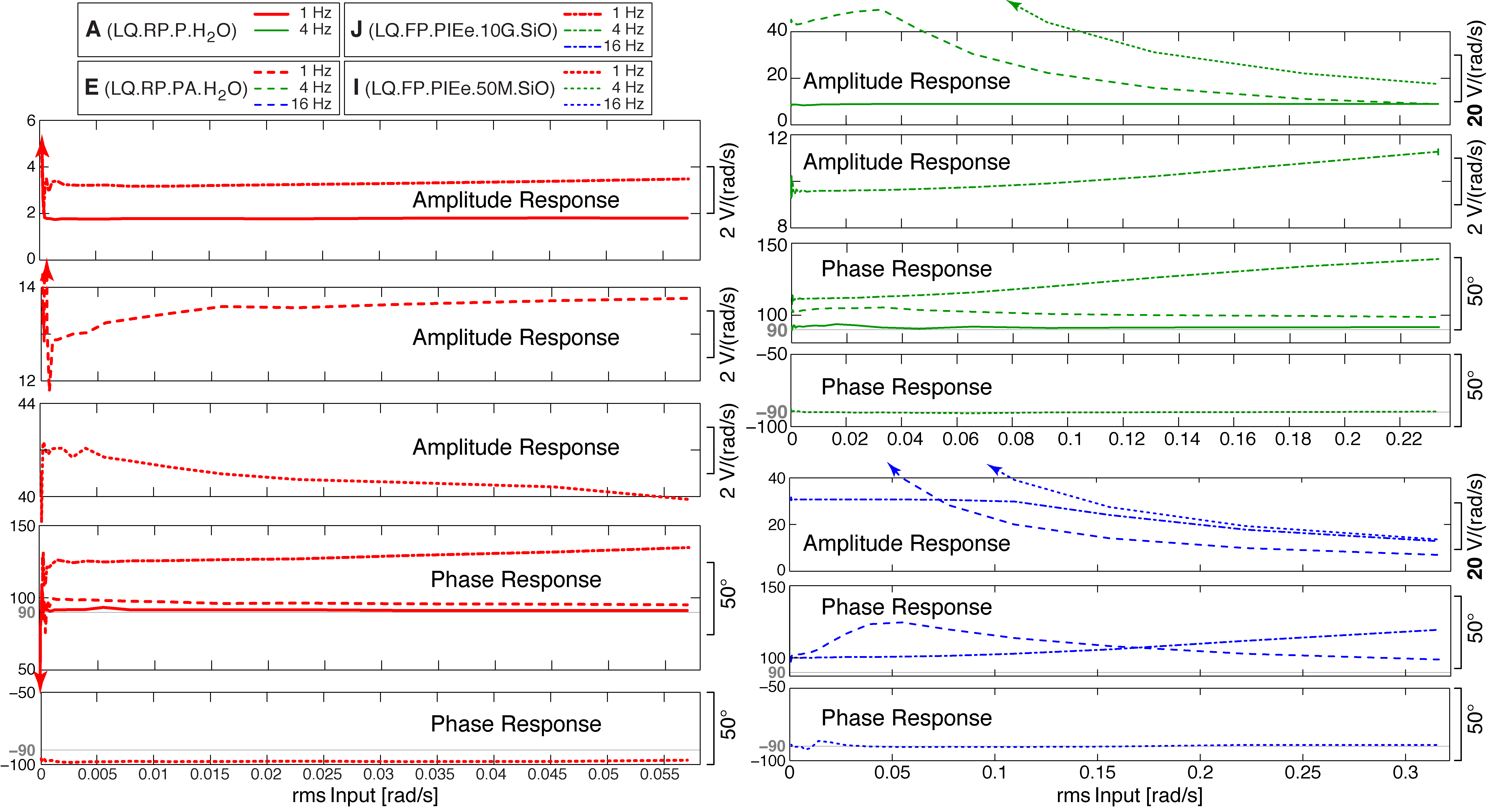
E (LQ.RP.PA.H2O): The TFF amplitude is more nearly proportional to acceleration than A, but has some sensitivity variation (e.g., 2.097 V/(rad/s2) at 1 Hz vs. 1.565 V/(rad/s2) at 8 Hz). E exhibits complexities from weak signals below about 0.6 Hz and a natural frequency near 40 Hz, particularly evident in phase; thus, it could reasonably be classified as a mixed-response combination.
J (LQ.FP.PIEe.10G.SiO): This combination is well behaved in the sense of having a smooth amplitude response and linear phase; however, the sensitivity varies over the tested range so that it is less than flat to acceleration at low frequencies but more than proportional at high frequencies (0.5824 V/(rad/s2) at 1 Hz vs. 0.3356 V/(rad/s2) at 8 Hz).
I (LQ.RP.PIEe.50M.SiO): Though their transition frequencies differ, this mass–transducer combination is similar to J in response but with better linearity over most of the tested frequency band (6.629 V/(rad/s2) at 1 Hz vs. 6.246 V/(rad/s2) at 8 Hz). Even so, frequencies above 10 Hz and below 0.3 Hz vary in amplitude response with frequency with no obvious natural-frequency signature in phase.
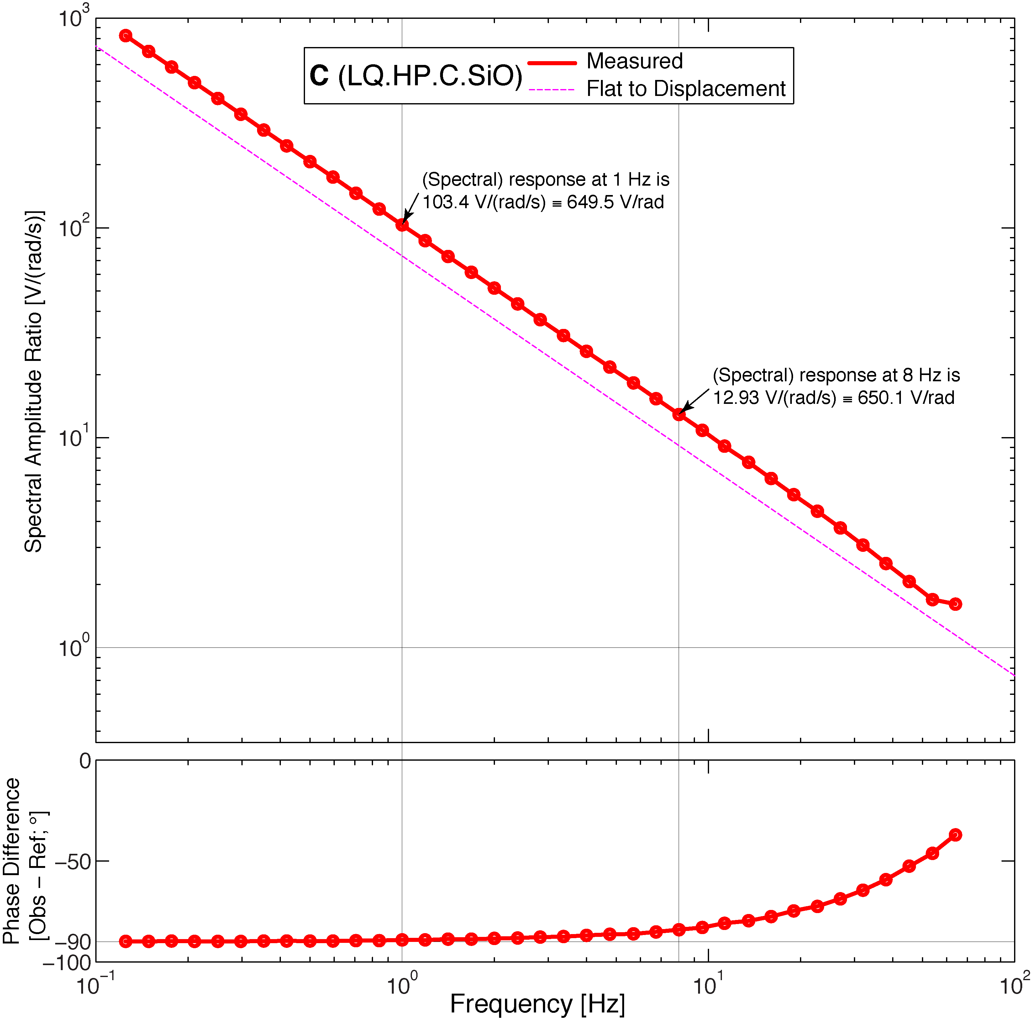
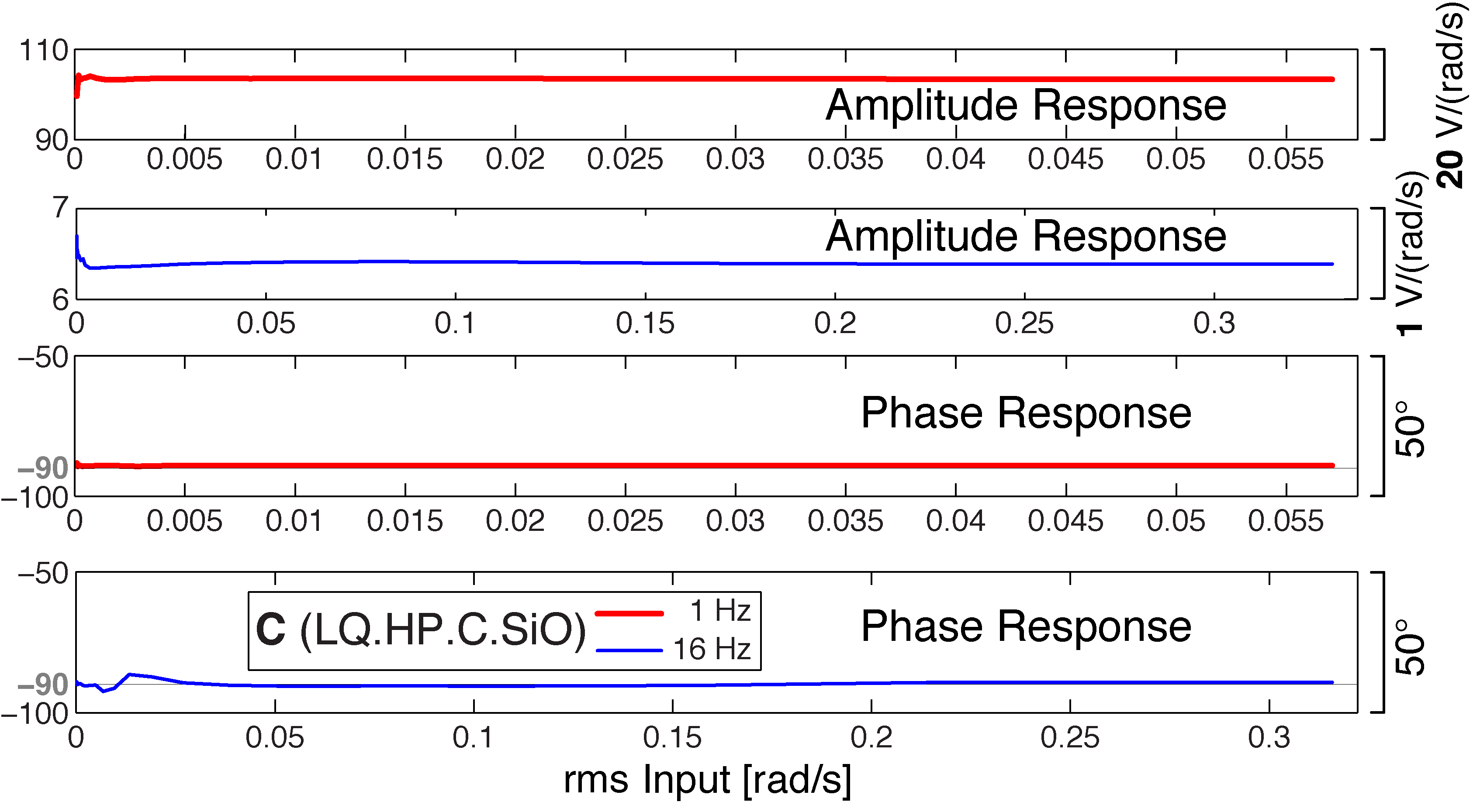
C (LQ.HP.C.SiO) is described in the main article.
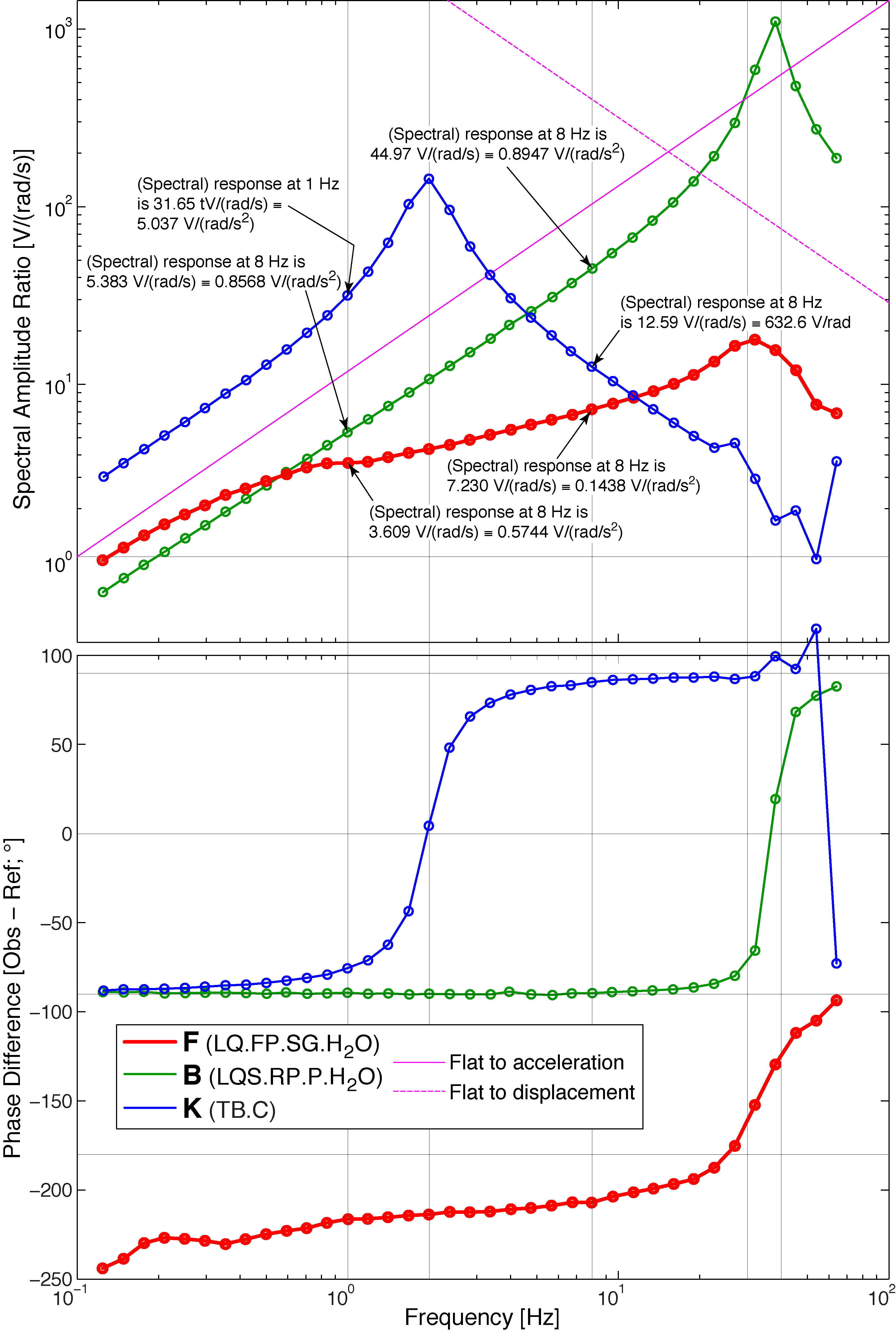
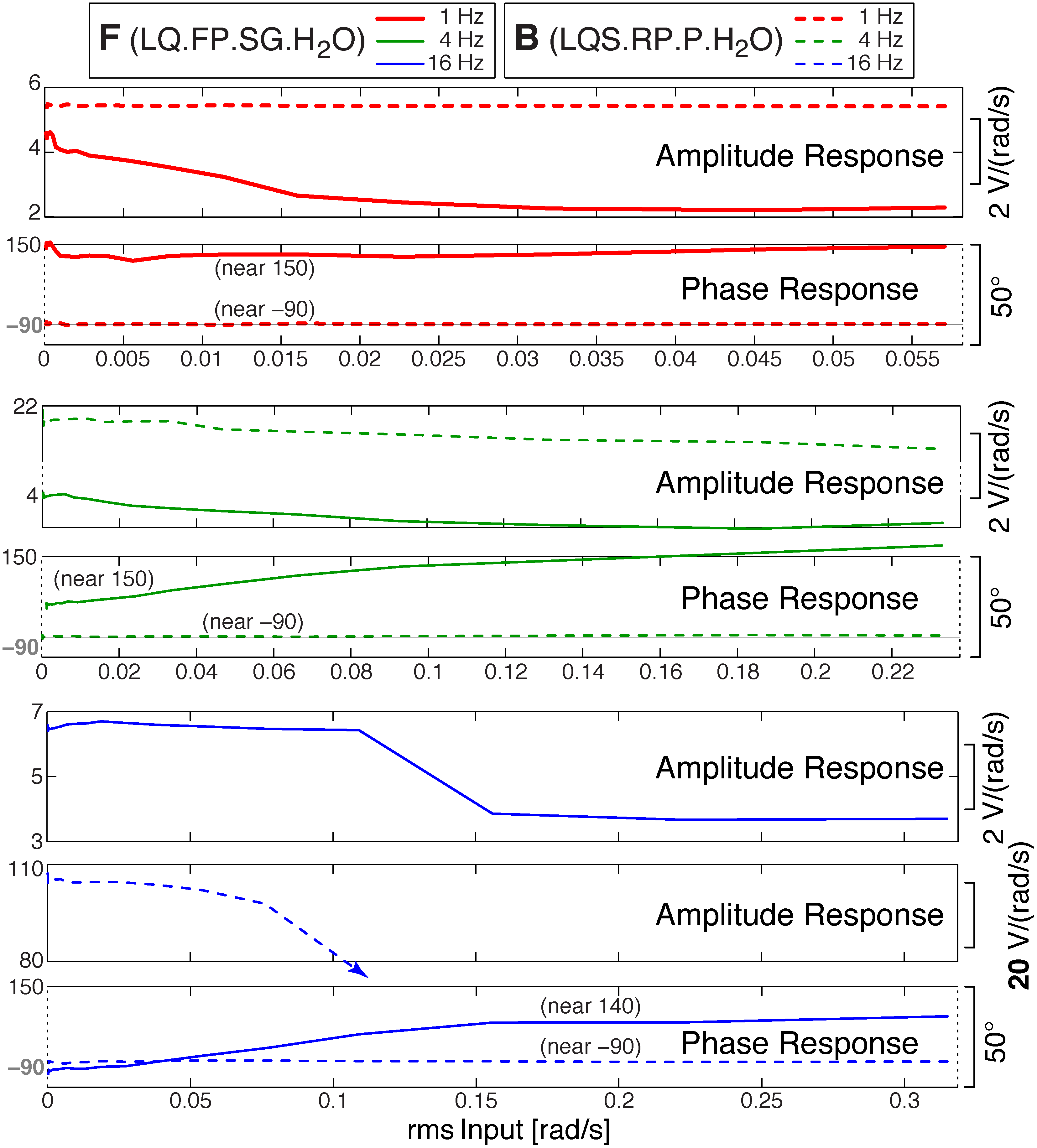
F (LQ.FP.SG.H2O): Most of the frequency range of this combination is more or less proportional to acceleration or some combination of acceleration and velocity, but there is a distinct natural frequency between 30 and 40 Hz and amplitude-response variations below about 1 Hz (0.5744 V/(rad/s2) at 1 Hz vs. 0.1438 V/(rad/s2) at 8 Hz). Output may be roughly proportional to displacement at high frequencies, but the limits of our test preclude proper evaluation.
B (LQS.RP.P.H2O) is described in the main article.
K (TB.C): This solid-mass sensor displays a sharply peaked amplitude response versus angular velocity and a 180° phase shift centered at the same frequency; thus, it has a natural frequency near 2 Hz and appears to be underdamped. Sensitivity below that frequency is about proportional to acceleration and above it is about proportional to displacement (5.037 V/(rad/s2) at 1 Hz vs. 632.6 V/rad at 8 Hz).
Amplitude means sensitivity, the ratio of output voltage divided by input rotational velocity (V/(rad/s)). Phase is that of the output voltage signal versus the input rotational-velocity signal.
A (LQ.RP.P.H2O) is described in the main article.
E (LQ.RP.PA.H2O) is roughly linear above 15 mrad/s at 1 Hz but not at other frequencies. Phase is nearly linear at +100°. At 4 and 16 Hz, amplitude is nonlinear everywhere, but at 4 Hz phase is the smoother of the two and near +100°. At 16 Hz, phase is quite nonlinear and somewhat higher than at 4 Hz.
J (LQ.FP.PIEe.10G.SiO) is roughly constant in amplitude and phase at 1 Hz and is also nearly linear below about 40 mrad/s at 4 Hz and below about 100 mrad/s at 16 Hz. Phase increases gently with increasing frequency at about +125° at 1 Hz, +110° at 4 Hz, and +100° at 16 Hz.
I (LQ.RP.PIEe.50M.SiO): Sensitivities are nonlinear except over a narrow range at 1 Hz. Phase is better behaved than sensitivity and is about −100° at 1 Hz and about −90° at 4 and 16 Hz.
C (LQ.HP.C.SiO) is described in the main article.
F (LQ.FP.SG.H2O): Amplitudes (sensitivities) are poorly behaved at all frequencies and at 16 Hz drop rapidly over the 110–160 mrad/s input range. Phase is nonlinear above 1 Hz and seems to range from about +140° to +160°.
B (LQS.RP.P.H2O) is described in the main article.
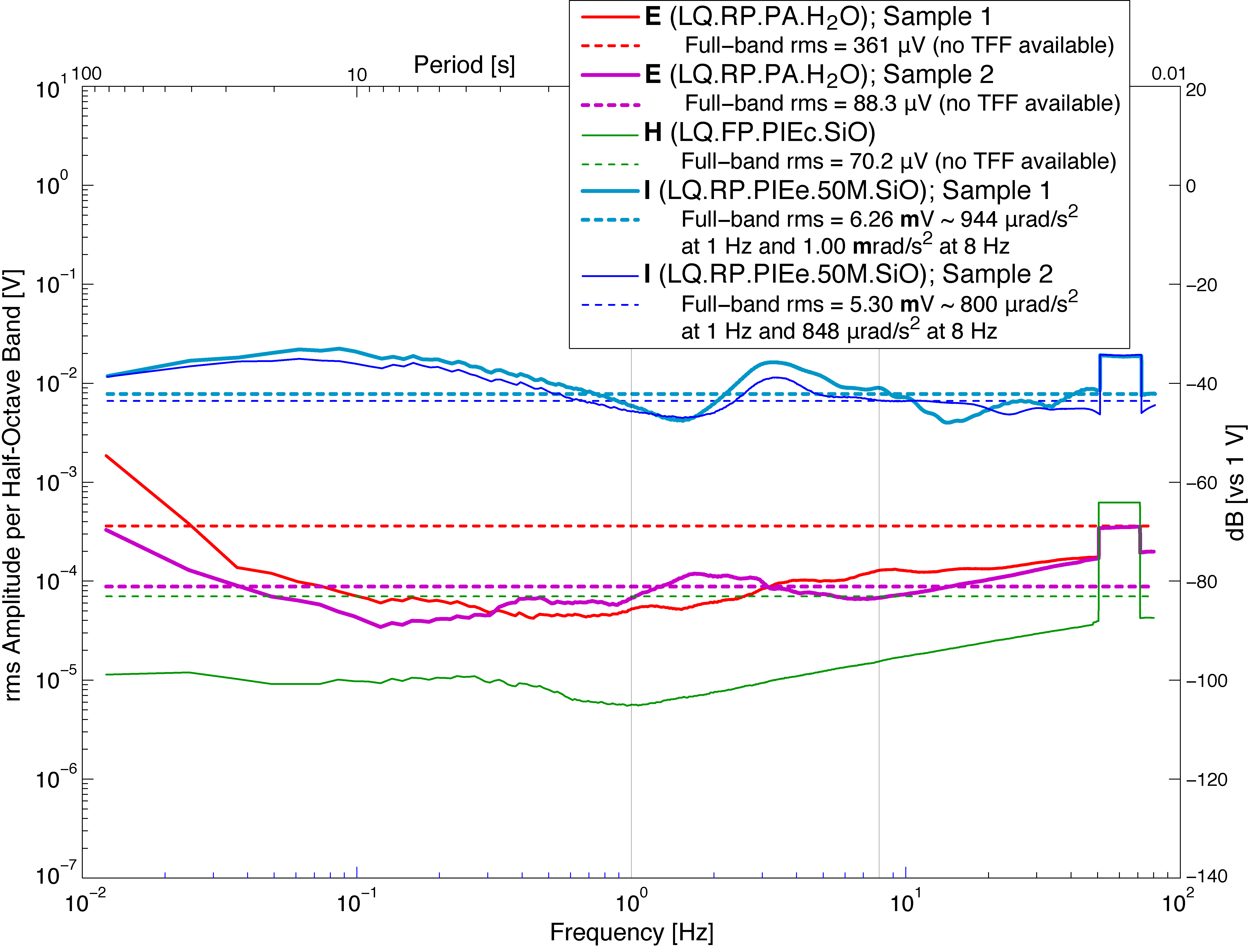
E (LQ.RP.PA.H2O): We tested two time intervals, so there are two results for this mass–transducer combination. In both tests, the time series (not shown) contains spikes, rapid groups of spikes, and offsets averaging about 1/100 s but not at constant intervals. The two samples have a full-bandwidth root mean square (rms) of 361 and 88.3 µV (no TFF is available), with the difference possibly caused by differing spike or offset patterns. The operating range diagrams (ORDs) are surprisingly well behaved given the time-series flaws and are roughly flat from 0.1 to 10 Hz, whereas they rise modestly on both sides of this range (Fig. S5a). Nevertheless, the time-series flaws are unacceptable in a deployed sensor.
H (LQ.FP.PIEc.SiO): Because we have no TFF for this combination either, we can only report that the output noise of the sensor is 70.2 µV and has a minimum near 2 Hz. If the sensitivity of this combination is similar to I, these would be low-noise values, but there is no guarantee of such equality.
I (LQ.RP.PIEe.50M.SiO): Again two time intervals were tested for this combination. Both time series had numerous spikes and sometimes steps associated with the spikes; as should be expected, the ORDs of both are very high but otherwise are similar to one another. They have full-bandwidth rms of 6.26 and 5.23 mV (at 1 Hz about 944 and 800 µrad/s2 and at 8 Hz about 1000 and 800 µrad/s2); these are very high values, as one would expect from the time-series flaws. Both the time series and the high-noise levels are unacceptable.
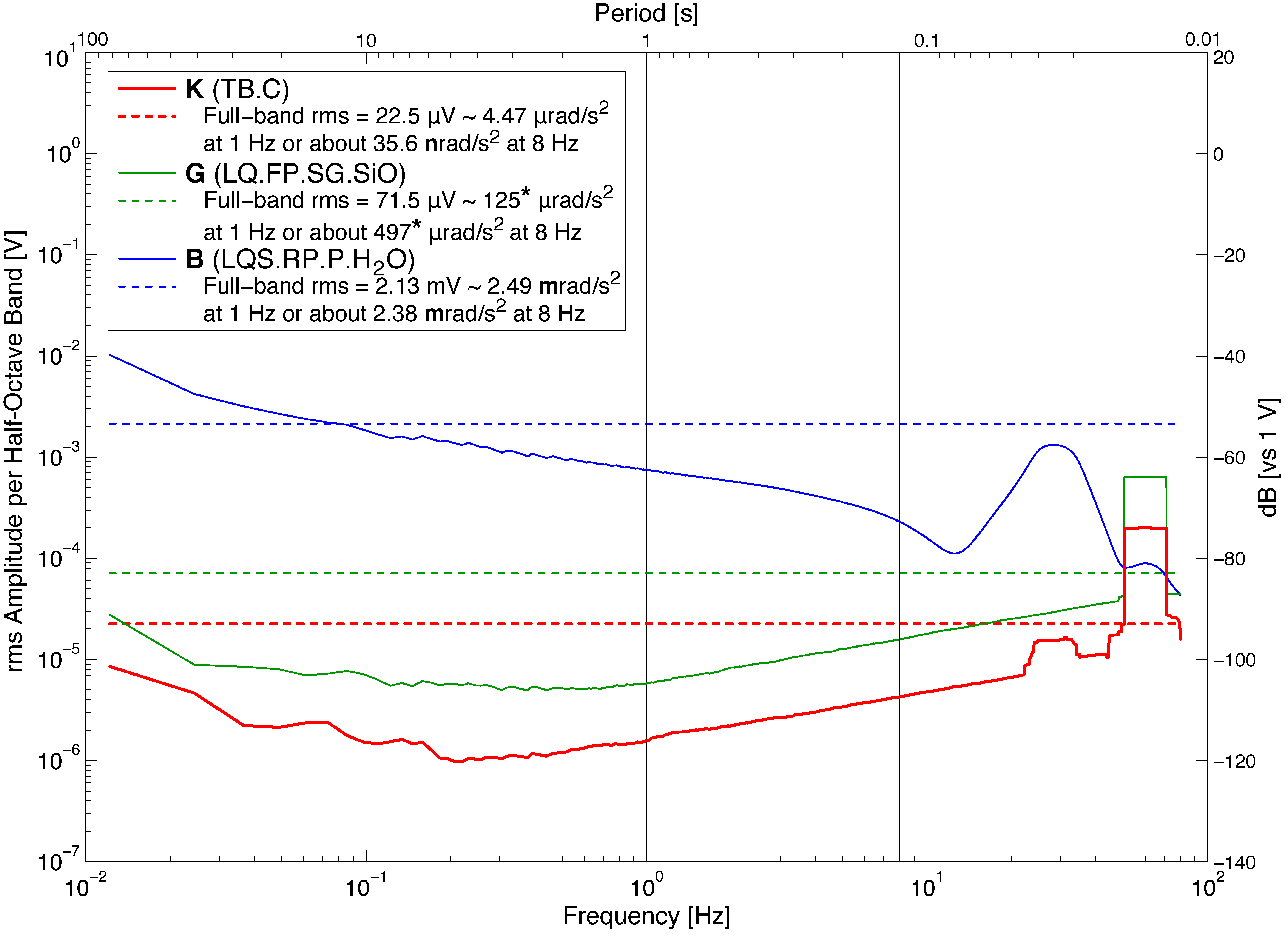
K (TB.C): This mass–transducer combination has good noise characteristics. Two time-series intervals were evaluated, with both well behaved, except for a single spike in one of them. The better of these two time series has a full-bandwidth rms near 22.5 µV (in the acceleration-proportional frequency range at 1 Hz equivalent to about 4.47 µrad/s2 and at 8 Hz in the displacement-proportional range about 35.6 nrad). These noise levels are quite low, but further shielding work may be called for.
G (LQ.FP.SG.SiO): The time series, mostly proportional to acceleration, is well behaved with no evident spikes or offsets. Its full-bandwidth rms is about 71.5 µV (about 125 and 497 µrad/s2 at 1 and 8 Hz); its well-behaved ORD has a minimum near 0.6 Hz. This mass–transducer combination and K appear to have the lowest, best-behaved noise signatures of the mixed-proportionality combinations tested.
B (LQS.RP.P.H2O) is described in the main article.
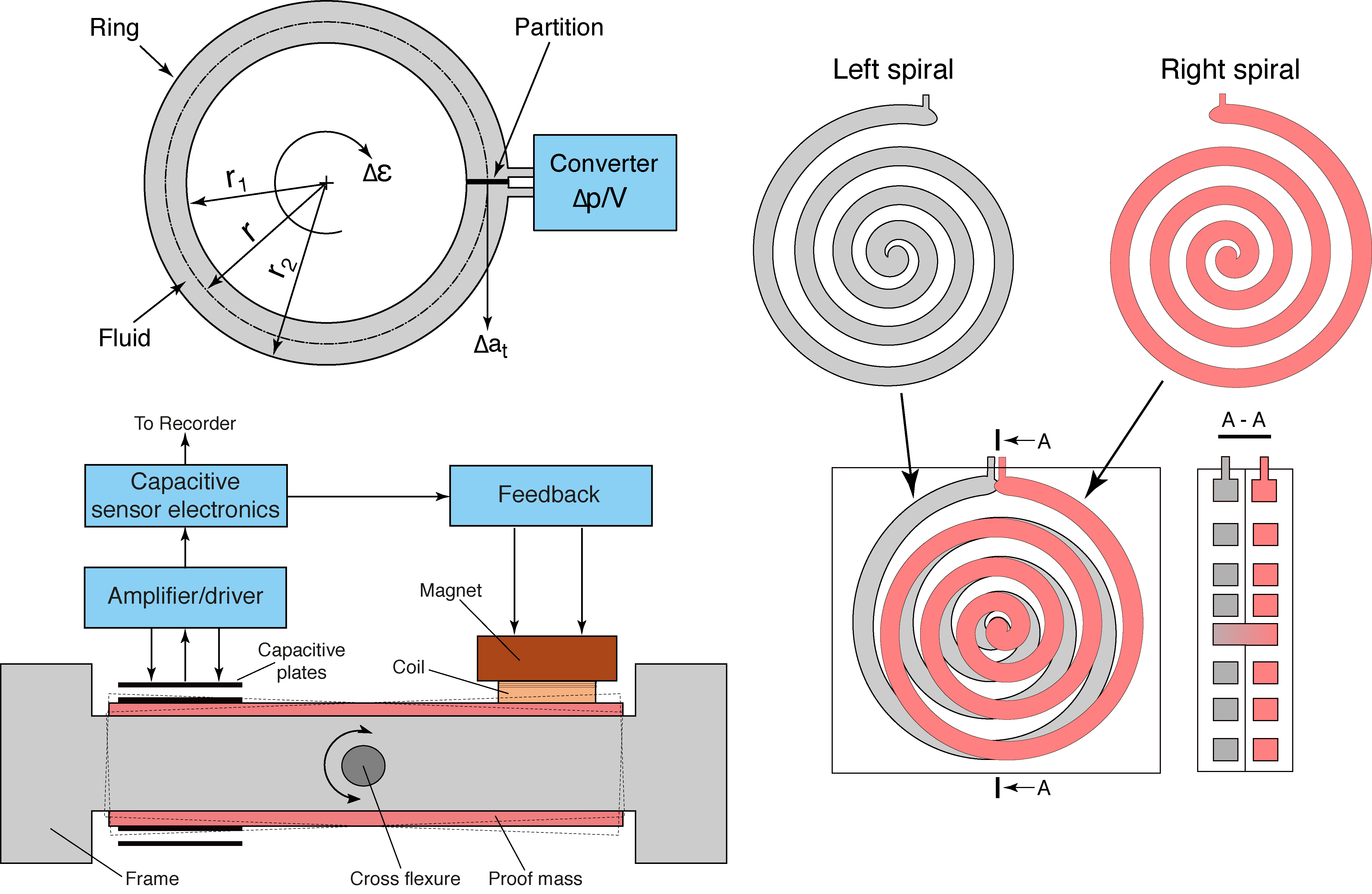
Figure S1. Drawings of liquid proof masses: (top left) the torus and (right, top, and bottom) the spiral. (Bottom left) the torsion bar solid proof mass with integrated capacitive transducer, amplifier, and electromagnetic feedback.
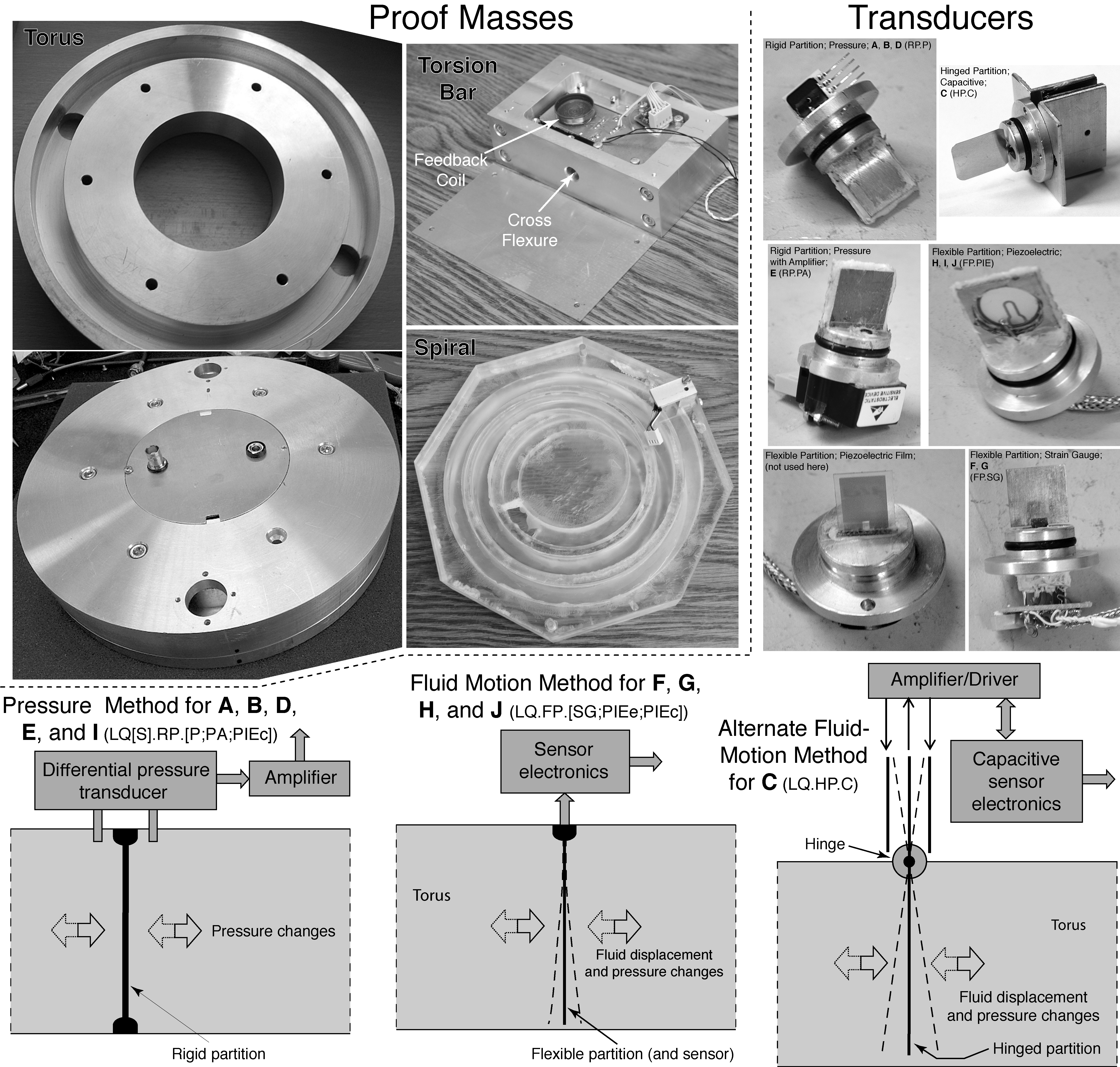
Figure S2. (top left) Photographs of the proof masses used. (right and bottom) Transducers that can be used with any of the fluid proof masses (water or silicon oil, and torus or spiral). (bottom left) A rigid partition spanned by pressure sensors; (bottom center) flexible partitions with integrated transducers; (bottom right) a hinged partition with external capacitive transducer.
Figure S3. Amplitude and phase TFFs divided into three groups: (a) combinations with output proportional to acceleration, (b) combinations with output proportional to angular displacement, and (c) combinations with mixed responses.
Figure S4. Clip and linearity tests for three frequencies of input sine waves, each for a range of input amplitudes (input-amplitudes necessarily vary by frequency to provide similar input velocities). The vertical axes are sensitivities (V/(rad/s)) or phase relative to input; horizontal axes are input sine amplitudes. (a) Results for 1-, 4-, and 16-Hz input signals for those mass–transducer combinations with outputs proportional to acceleration. (b) Same for (a) but for the only combination with outputs proportional to displacement. (c) Same as for (a) but for the three combinations with outputs proportional to a mix of acceleration and displacement.
Figure S5. Noise plots presented as ORDs (rms per half-octave) and full-bandwidth rms values (dashed lines of same color). Note that full-bandwidth rms includes the often large effects of high-frequency spikes in the power spectral density (PSD; not shown; e.g., H), and the effects of the 2-Hz peak seen in the results for E. (a) Combinations with TFFs proportional to acceleration and (b) those with mixed acceleration-displacement responses. Mesa-like features at high frequency are due to narrowband electromagnetic interference (spikes) common at this laboratory; the spikes are broadened by the running half-octave sum of the PSD required to compute the ORD; they should be ignored.
[ Back ]