This electronic supplement contains figures of QP and QS resolution and station delays for t*, and Table S1 of QP, VP, QS, and VS. The method for fitting t* to earthquake spectra is described in Figure S1. The resolution of the 3D models is shown by the spread function (SF) in Figures S2 and S3, for all depths. The station t* terms are shown in Figure S4, and they are quite small, because most heterogeneity is included in the 3D models.
Table S1 [Plain Text Comma-separated Values; ~4.1 MB]. Table S1 contains the northern California 3D attenuation model parameters QP and QS and associated VP and VS, following Lin et al. (2010). The spatial resolution and data distribution are described by the SF (Michelini and McEvilly, 1991), where lower value is better resolution and values over 4.0 indicate poor resolution, no data at 6.0, and peripheral nodes at 8.0. Cartesian coordinates x and y are for the rotated grid shown in Figure 1 of the main article, with origin at 36.5° N, 120.0° W, and distances are converted using transverse Mercator with central meridian of 121.5° W. Depth is in kilometers below sea level. The table contains peripheral values that extend the x and y grids by 300 km. This is done so that the model will be easier to implement for earthquakes and stations that are outside the area but have useful ray paths in northern California.
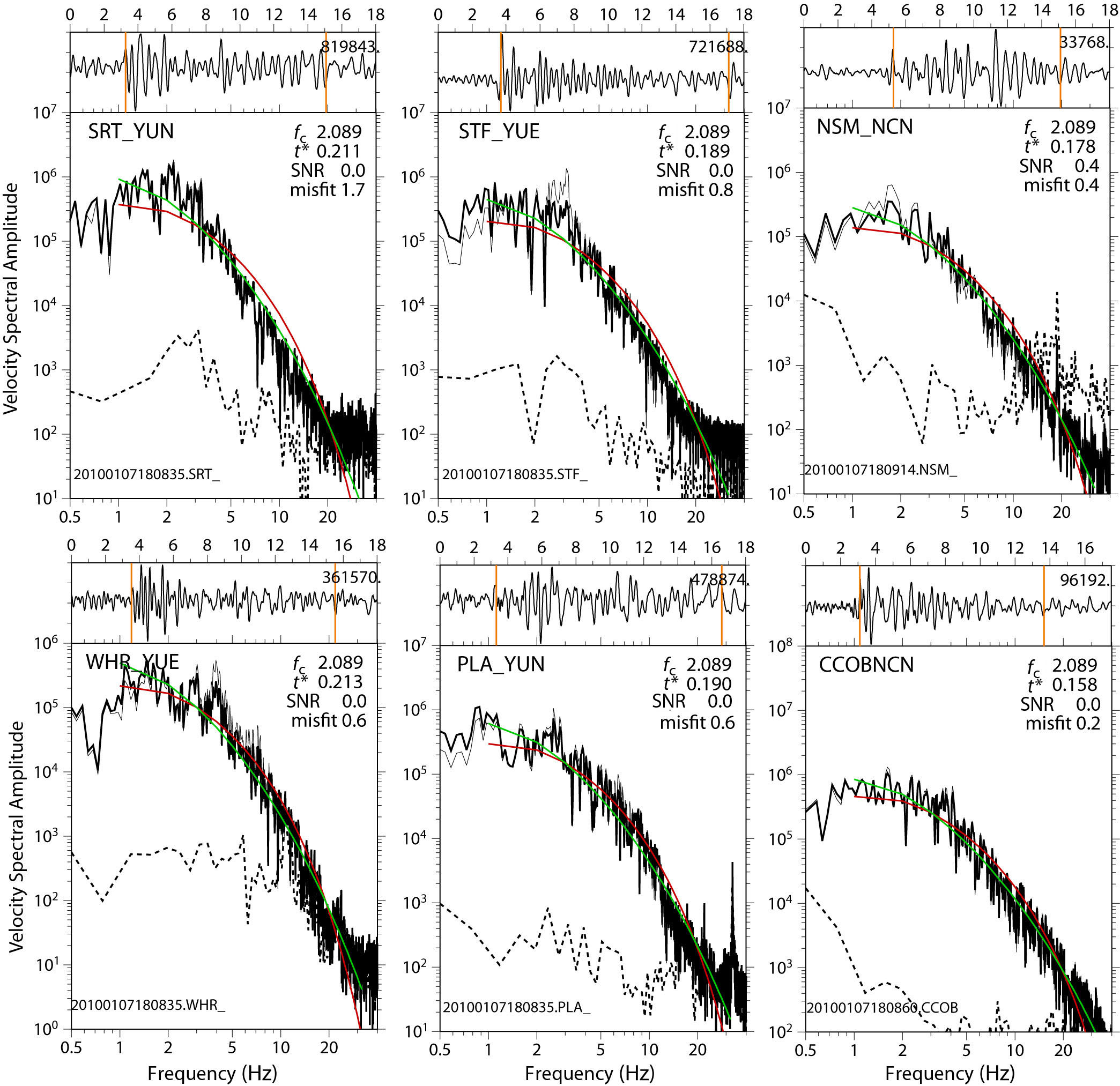
Figure S1. An example of t* fitting for the energy-integral S, comparing the frequency-independent and α = 0.5 frequency-dependent results, for an M 4.3 earthquake on the Calaveras fault. In each plot, the frequency independent is the most bent line. The labeled t*, fc, signal-to-noise ratio (SNR), and misfit are for the α = 0.5 (f0 = 10 Hz) results. The thin line shows the initial spectra; the thick line shows the spectra after removal of site response; and the dashed line is the noise spectra.
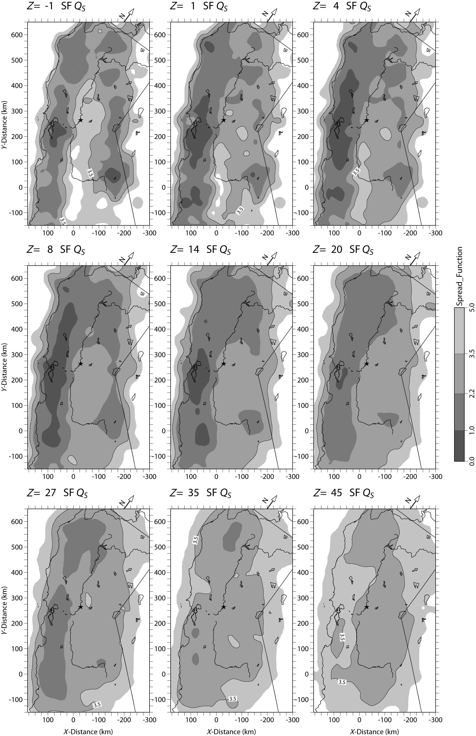
Figure S2. Plots of resolution as indicated by SF for 3D QS, for all model depths −1 to 45 km.
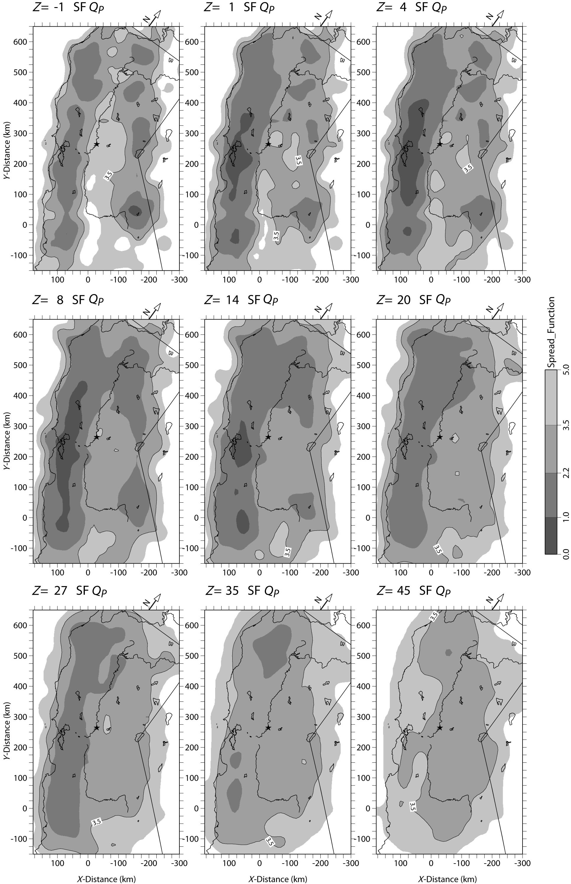
Figure S3. Plots of resolution as indicated by SF for 3D QP, for all model depths −1 to 45 km.
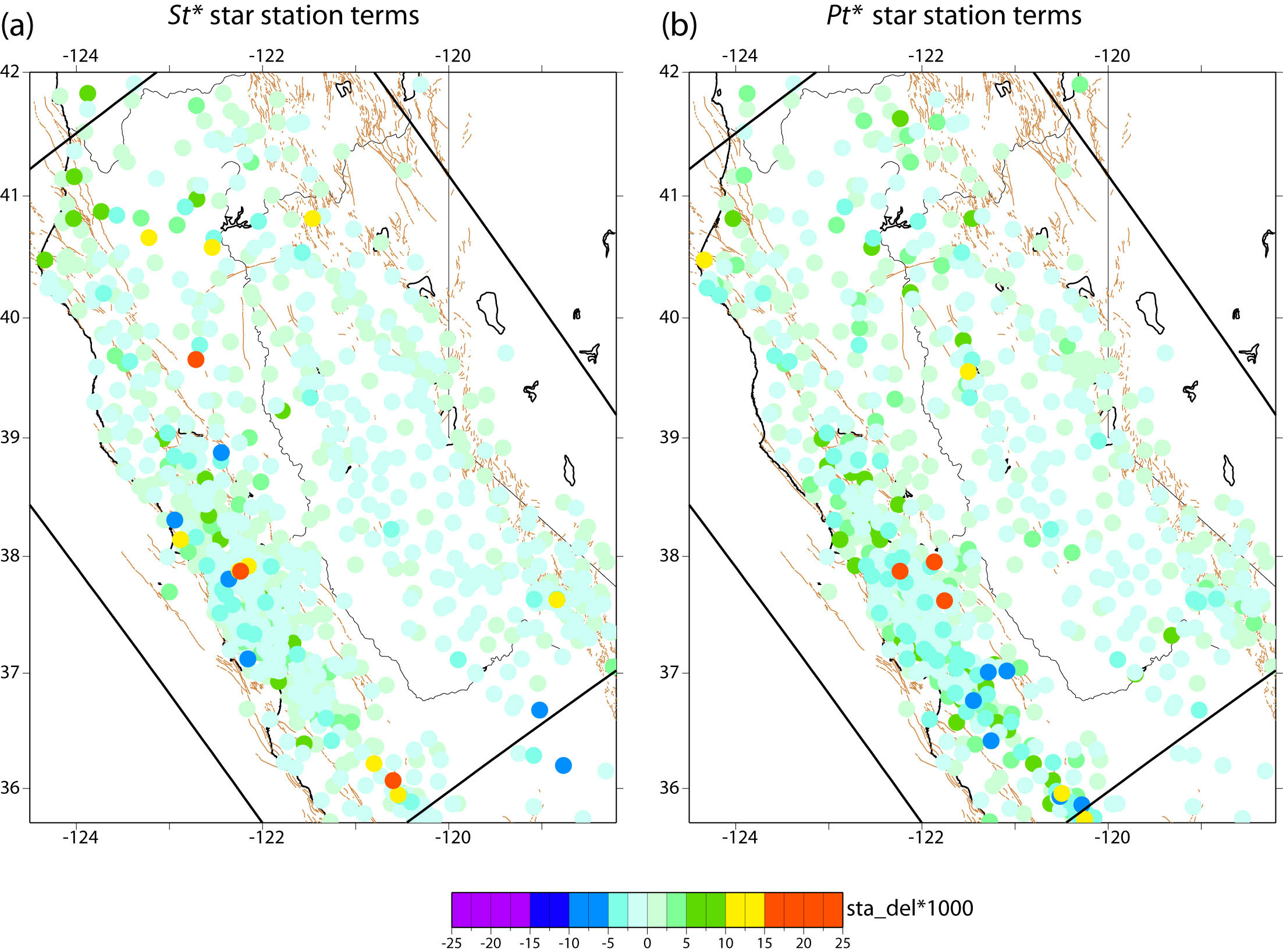
Figure S4. Station delays for t* were included in the 3D inversion, for (a) S and (b) P.
Lin, G., C. H. Thurber, H. Zhang, E. Hauksson, P. M. Shearer, F. Waldhauser, T. M. Brocher, and J. Hardebeck (2010). A California statewide three-dimensional seismic velocity model from both absolute and differential times, Bull. Seismol. Soc. Am. 100, 225–240, doi: 10.1785/0120090028.
Michelini, A., and T. V. McEvilly (1991). Seismological studies at Parkfield: I. Simultaneous inversion for velocity structure and hypocenters using cubic b-splines parameterization, Bull. Seismol. Soc. Am. 81, 524–552.
[ Back ]