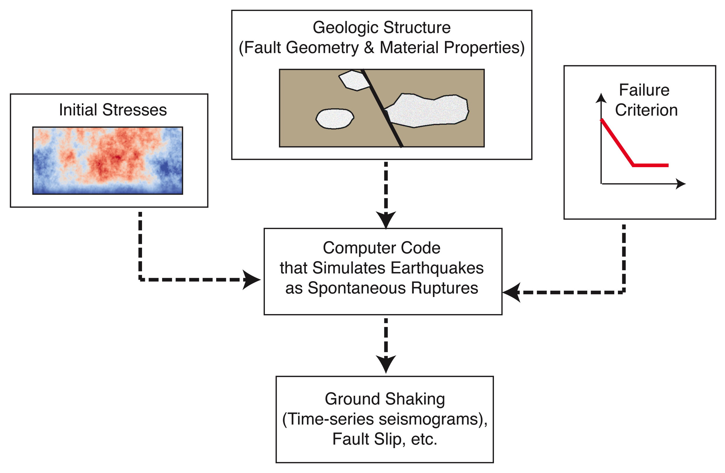
A dynamic rupture simulation is a numerical model of the physical processes that occur during an earthquake. The model consists of the fault geometry, rock constitutive properties, friction constitutive law, boundary conditions, and initial conditions. The computer integrates the model forward in time to calculate the earthquake nucleation, the evolution of fault slip and stress as the rupture spreads across the fault surface, and the resulting seismic waves (Fig. S1).
For most of our benchmarks, the geometry is a semi-infinite half-space, which contains one or more fault surfaces. The geometry remains fixed during the simulation.
Rock deformation is represented by a vector-valued displacement field uα that varies with position and time. The index α runs over the three coordinate directions x, y, and z. The vector uα is the displacement of the rock from its initial position. The displacement field is continuous everywhere except on the fault surface. A discontinuity in the displacement field represents fault slip. The fault slip vector sα is defined as the difference in the values of uα on the two sides of the fault, sα ≡ . In our benchmarks, the fault slip vector is required to be tangent to the fault surface, which means that the fault is not allowed to open.
The displacement is assumed to be small, so we use the infinitesimal strain tensor, which is eαβ ≡ (uα,β + uβ,α)/2. A subscript comma indicates differentiation, so uα,β ≡ ∂uα / ∂xβ. The time derivatives , and are the velocity field, the slip rate vector, and the strain rate tensor, respectively.
Stresses in the rock are represented by the stress tensor σαβ, which varies with position and time. Rock constitutive properties specify how the stress tensor can be computed from the strain and strain rate tensors. In principle, the value of the stress tensor can depend on the entire past history of the strain and strain rate tensors. In practice, the computer encodes the strain history in a small number of state variables, which are integrated forward in time as part of the simulation. The stress tensor can then be computed from the state variables and the current values of the strain and strain rate tensors.
The majority of our benchmarks use linear elastic rock properties, in which the stress tensor depends on the strain tensor and two constitutive parameters λ and μ:
σαβ = λδαβeγγ + 2μeαβ.
(S1)
The symbol δαβ is the Kronecker delta, and repeated indices are summed. Some of our benchmarks use plastic or viscoplastic rock constitutive properties, which are considerably more complicated.
At the Earth’s surface, the stress tensor must satisfy the free-surface boundary condition , where is the normal vector to the free surface. Although the model is semi-infinite, many computer codes must restrict the computation to a domain of finite size. When a finite domain is used, the code must impose suitable boundary conditions at the edges of the domain, which are typically designed to reduce reflections of seismic waves from the boundaries.
The traction force acting on the fault surface is Tα ≡ σαβnβ, where nβ is the normal to the fault surface. The normal and tangential components of the vector Tα correspond to the normal and shear stresses on the fault surface. The traction force must satisfy two boundary conditions: the value of Tα must be the same on both sides of the fault surface, and the tangential component of −Tα must equal the friction force. This implies that Tα is parallel to the slip rate vector, because friction is antiparallel to the direction of slip.
Friction constitutive laws specify how the friction force can be computed from the normal stress and slip rate. Analogously to rock constitutive properties, the friction can in principle depend on the entire past history of normal stress and slip rate. In practice, the computer encodes the history in a small number of state variables, which are integrated forward in time as part of the simulation. The friction force can then be computed from the state variables and the current values of normal stress and slip rate.
The majority of our benchmarks use linear slip weakening friction. The slip history is encoded in a variable D, which is the path-integrated total slip distance since the start of the simulation. The linear slip weakening relation is
τ = σeff [μs + (μd − μs) min (D/d0,1)] + C0,
(S2)
in which τ is the magnitude of the friction force, σeff is the effective normal stress (usually defined to be normal stress minus pore pressure, and not to be confused with the stress tensor), μs is the static coefficient of friction, μd is the dynamic coefficient of friction, d0 is the critical slip distance, and C0 is the frictional cohesion. Some of our benchmarks use rate–state friction, which is more complicated and explicitly depends on slip rate.
The elastodynamic wave equation, which governs the propagation of seismic waves, is
ρ = σαβ,β − ρg
(S3)
in which ρ is density, g is the acceleration due to gravity, and is an upward-pointing unit normal vector. In order to integrate the dynamic rupture simulation forward in time, the computer code must solve the elastodynamic wave equation simultaneously with the rock constitutive properties, the friction constitutive laws, and the boundary conditions.
To begin the simulation, it is necessary to specify initial conditions. The initial displacement field uα is zero by definition. The initial velocity field is usually taken to be zero, however some rate–state friction laws require a small nonzero initial velocity. The initial stress tensor σαβ is usually taken to be in static equilibrium. For linear elastic models, it is sufficient to specify the initial traction force Tα instead of the initial stress tensor. It is also necessary to specify initial values for any state variables that appear in the rock constitutive properties or friction constitutive laws.
Finally, in order to start the earthquake rupture, there must be some artificial nucleation mechanism. Often the rupture is nucleated either by imposing a high initial shear stress near the hypocenter or by artificially reducing the friction force near the hypocenter.
There are several numerical methods available for solving these coupled nonlinear differential equations, including finite element, finite difference, boundary integral, and spectral element methods. Details of some methods can be found in Andrews (1999), Day et al. (2005), Ma and Liu (2006), Dalguer and Day (2007), and Barall (2009). Additional references can be found on our project website at http://scecdata.usc.edu/cvws (last accessed November 2014).
Figure S1. Dynamic (spontaneous) rupture simulations of earthquakes require assumptions about the fault geometry, the initial stress conditions, the boundary conditions, the physical characteristics of the off-fault rocks and how they respond to stressing, and a failure criterion or friction law that determines if a part of the fault can slip and at what level of frictional force. The computer code calculates the full inertial dynamics and wave propagation, in addition to the physics of earthquake faulting. The simulation can produce many types of results, including synthetic seismograms, fault slip histories, earthquake magnitude and extent, and a wealth of additional information.
Andrews, D. J. (1999). Test of two methods for faulting in finite-difference calculations, Bull. Seismol. Soc. Am. 89, no. 4, 931–937.
Barall, M. (2009). A grid-doubling finite-element technique for calculating dynamic three-dimensional spontaneous rupture on an earthquake fault, Geophys. J. Int. 178, 845–859, doi: 10.1111/j.1365-246X.2009.04190.x.
Dalguer, L. A., and S. M. Day (2007). Staggered-grid split-node method for spontaneous rupture simulation, J. Geophys. Res. 112, no. B02302, doi: 10.1029/2006JB004467.
Day, S. M., L. A. Dalguer, N. Lapusta, and Y. Liu (2005). Comparison of finite difference and boundary integral solutions to three-dimensional spontaneous rupture, J. Geophys. Res. 110, no. B12307, 23 pp., doi: 10.1029/2005JB003813.
Ma, S., and P. Liu (2006). Modeling of the perfectly matched layer absorbing boundaries and intrinsic attenuation in explicit finite-element methods, Bull. Seismol. Soc. Am. 96, no. 5, pp. 1779–1794, doi: 10.1785/0120050219.
[ Back ]