This electronic supplement contains a larger set of test results than the main article, all the formulas and parameter values used to construct our three model fault surfaces, step-by-step algorithms for constructing fault discretizations, and additional figures showing the fault geometry and the source and target regions of our tests.
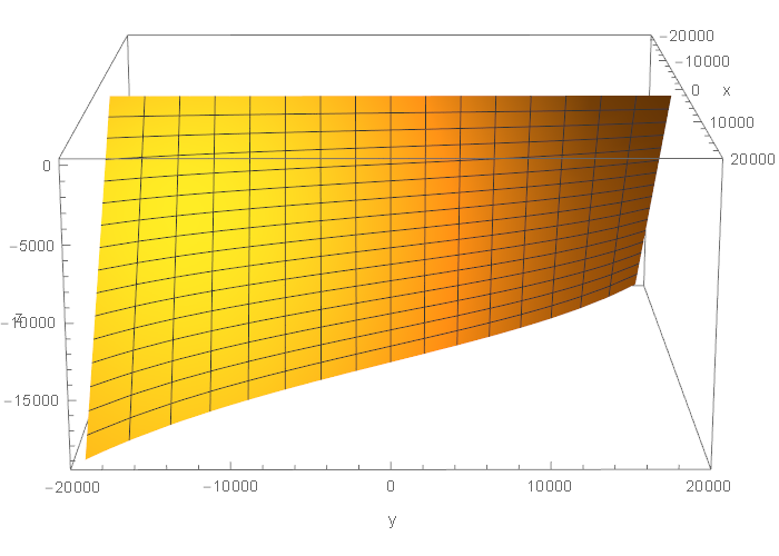
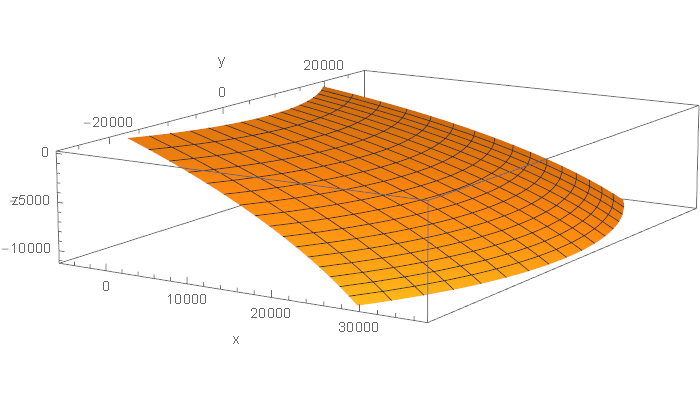
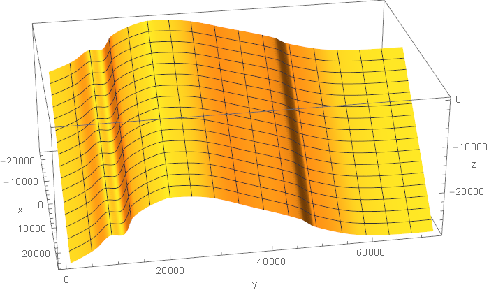
Our negatively curved fault surface is a section of a helicoid. It is a strike-slip fault. Figure S1 shows the fault surface. The following equations show the mapping from () coordinates (in which is depth and is distance along strike) to () coordinates that defines the shape of the fault surface. Table S1 shows the values of the parameters appearing in these equations.
We present test results for four configurations of source and target regions, which we denote N1–N4. Table S2 defines the four combinations of source and target regions used in our tests of the negatively curved (helicoidal) fault surface. Figures S2–S5 show configurations N1–N4, respectively. Configurations N1 and N2 are the ones used in the main article.
We use three discretization patterns for the negatively curved surface, denoted “rectangle,” “triangle-2,” and “triangle-4.” To produce the rectangle discretization, we perform the following steps:
To produce the triangle-2 discretization, we perform the following steps:
To produce the triangle-4 discretization, we perform the following steps:
Our positively curved fault surface is a section of an ellipsoid. It is a dip-slip fault. Figure S6 shows the fault surface. The following equations show the mapping from () coordinates (in which is depth and is distance along strike) to () coordinates that defines the shape of the fault surface. Table S3 shows the values of the parameters appearing in these equations.
We present test results for three configurations of source and target regions, which we denote P1–P3. Table S4 defines the three combinations of source and target regions used in our tests of the positively curved (ellipsoidal) fault surface. Figures S7–S9 show configurations P1–P3, respectively. Configurations P1 and P2 are the ones used in the main article.
We use three discretization patterns for the positively curved surface, denoted rectangle, triangle-1, and triangle-3. To produce the rectangle discretization, we perform the following steps:
Notice that, because each strip has a different length and a different number of rectangles, the rectangles do not produce a checkerboard pattern. In other words, a vertex of a rectangle can lie in the middle of an edge of a rectangle in an adjacent strip. So, unlike our negatively curved fault, it is not possible to triangulate the surface by starting with rectangles and then cutting the rectangles into triangles.
To produce the triangle-1 and triangle-3 discretizations, we perform the following steps:
Our zero-curvature fault surface is a section of a cylinder with an irregular cross section. It is a dip-slip fault, which has the actual shape of the North Frontal West fault. Figure S10 shows the fault surface. The following equations show the mapping from () coordinates (in which is depth and is distance along strike) to () coordinates that defines the shape of the fault surface.
Table S5 shows the values of the parameters appearing in these equations. The arc midpoint of the fault trace is located at . The file NFW_UCERF3_FM3_2.zip contains the geometry of the North Frontal West fault, as described by Uniform California Earthquake Rupture Forecast, Version 3 (UCERF3) fault model v.3.2. File NFW_Interpolated.zip contains the values of the function and the rake angles, tabulated at intervals of 10 m, which we computed by interpolating the UCERF3 waypoints.
The interpolated values are calculated using Hermite interpolation of order 3. Hermite interpolation requires a function value and slope at each waypoint. At each waypoint other than the first and last, the slope equals the slope of the line connecting the previous waypoint to the next waypoint. At the first waypoint, the slope equals 1.5 times the slope of the line connecting the first and second waypoints, minus 0.5 times the slope of the line connecting the first and third waypoints. This is as close as possible to the slope of the line connecting the first and second waypoints, without creating an inflection point. The last waypoint is handled similarly. Finally, we add two new waypoints, located about 20 km beyond each end of the fault trace and with zero slope, so that the interpolated fault trace continues smoothly beyond the endpoints. This is for the benefit of discretization algorithms that need to sample points somewhat beyond the ends of the fault trace.
Rake angles are computed by assuming that fault slip is parallel to the cylinder axis. The cylinder axis is specified by the dip angle and dip direction given in the UCERF3 fault model.
We present test results for three configurations of source and target regions, which we denote C1–C3. Table S6 defines the three combinations of source and target regions used in our tests of the zero-curvature (cylindrical) fault surface. Figures S11–S13 show configurations C1–C3, respectively. Configurations C1 and C2 are the ones used in the main article.
We use four discretization patterns for the zero-curvature surface. The rectangle, triangle-1, and triangle-3 discretizations are constructed using the same procedure as for the positively curved (ellipsoidal) fault surface. To produce the triangle-4 discretization, we perform the following steps:
We do not use the triangle-2 discretization, because in this case it would be the same as triangle-1.
As noted above, in order to discretize a curved fault surface with rectangles, it is necessary to modify the original nonplanar quadrilaterals to form rectangles that are suitable for use with the Okada formulas. We are not aware of a published standard algorithm for performing this modification, although it is likely that modelers have created such algorithms for their own use, so we created an algorithm, which we describe here.
Starting with a nonplanar quadrilateral, the four vertices of which lie in the fault surface, we perform the following steps to convert it into a suitable rectangle:
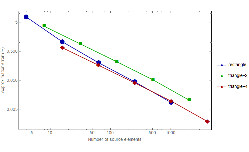
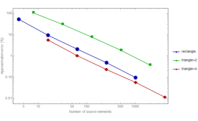
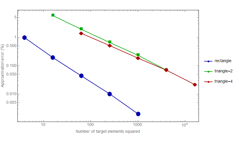
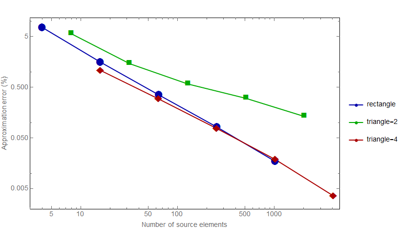
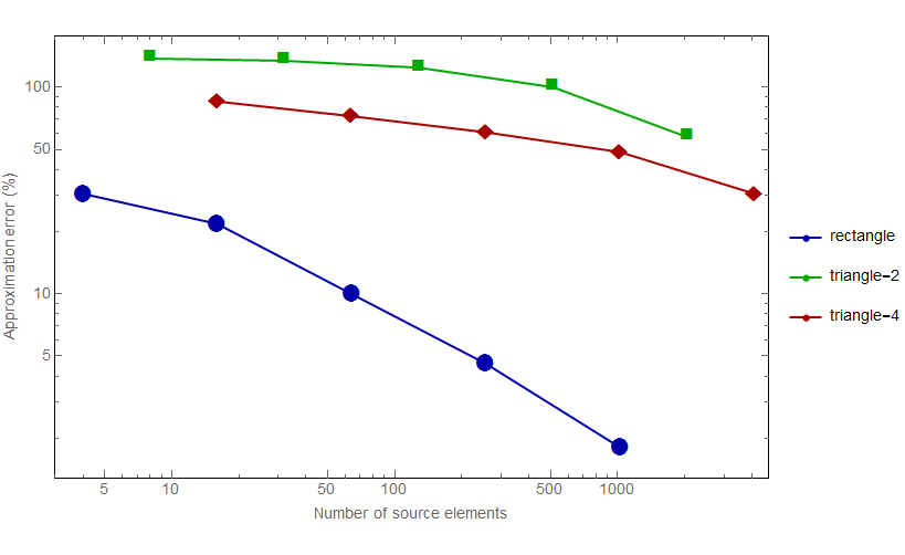
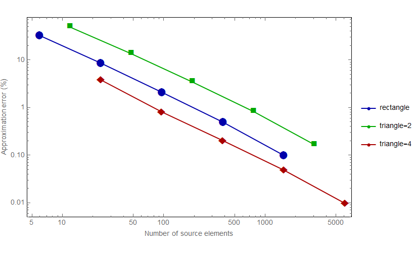
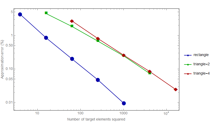
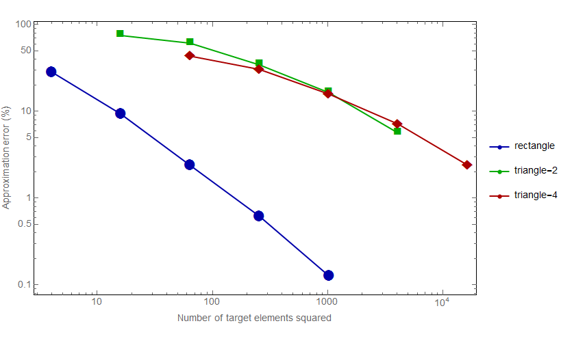
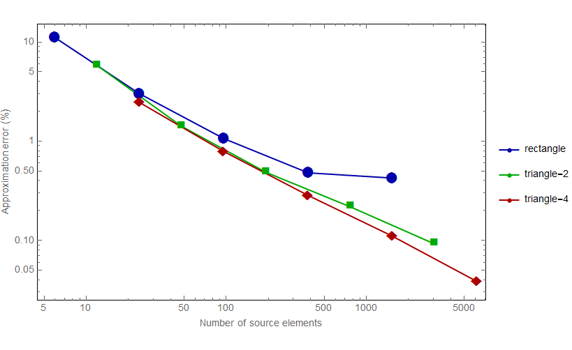
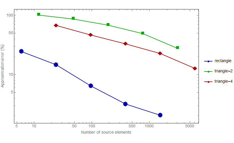
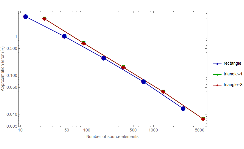
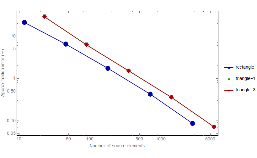
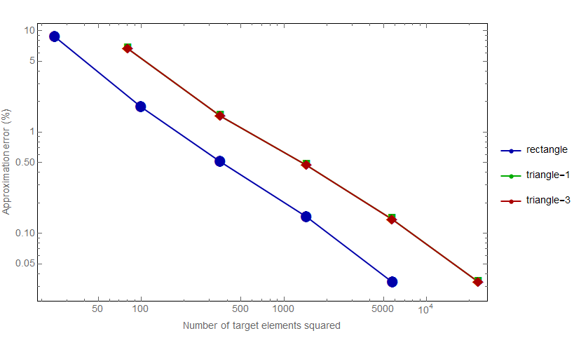
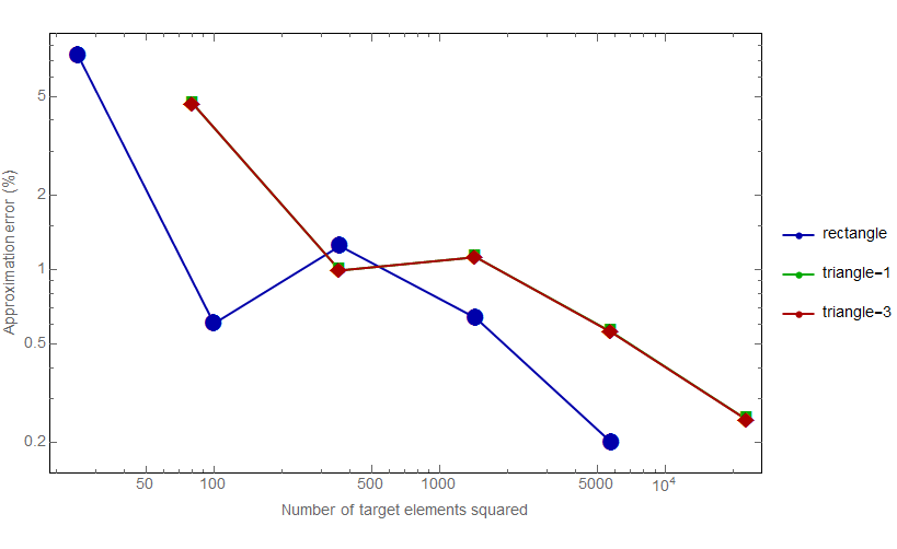
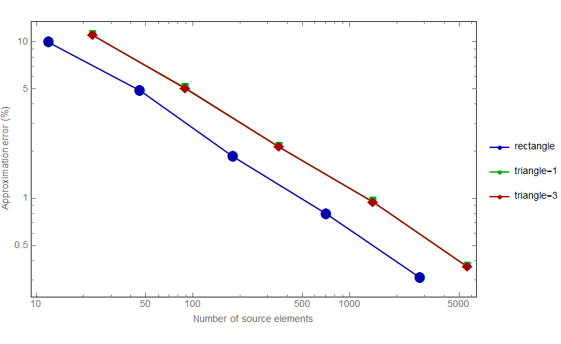
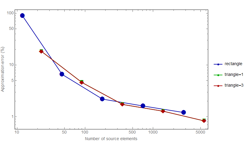
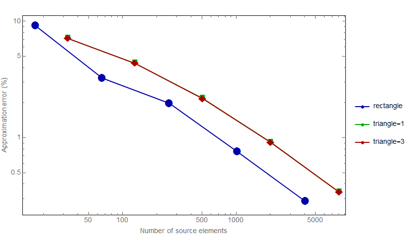
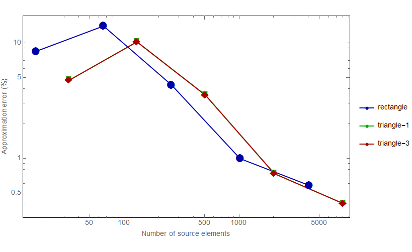
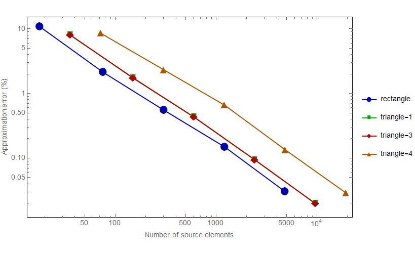
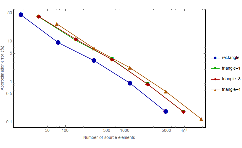
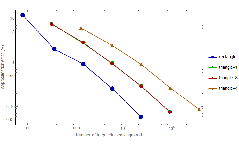
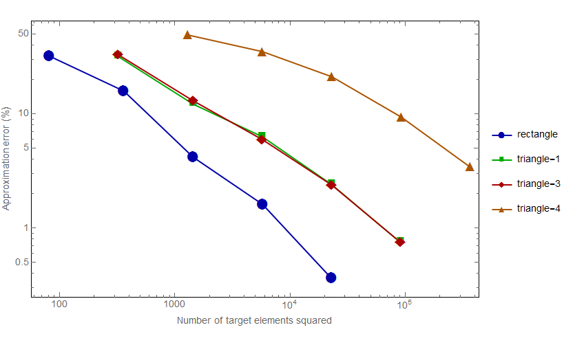
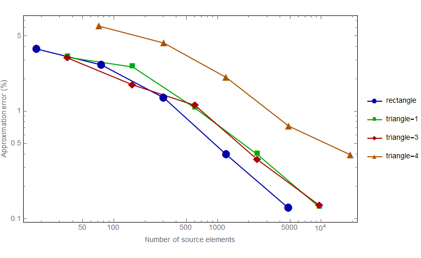
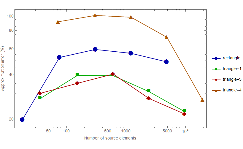
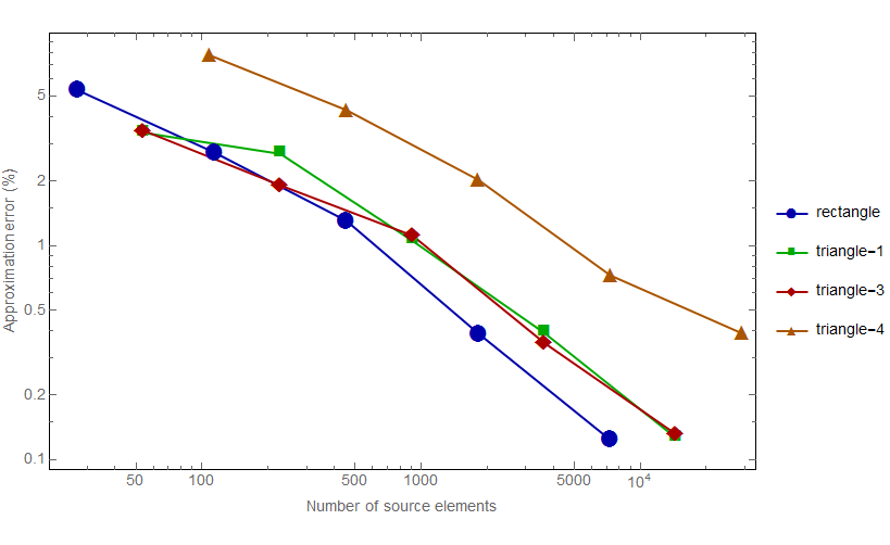
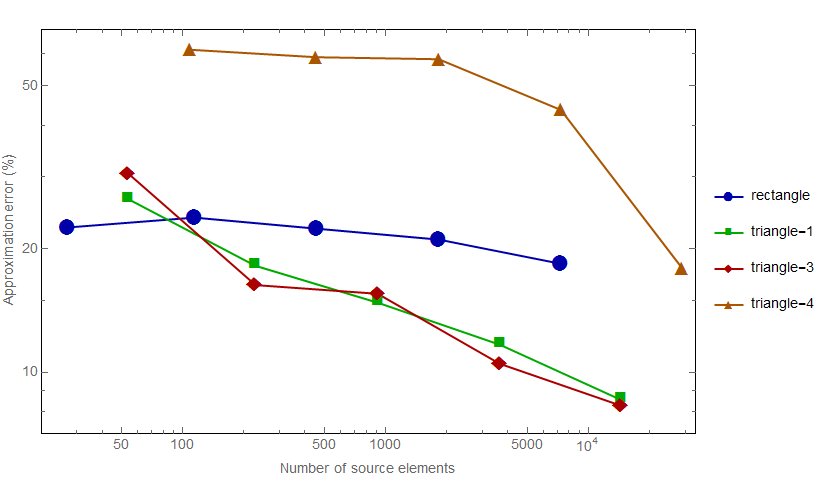
Our test results are presented in graphical form. The graphs show how the accuracy of the stress calculation varies as the size of the fault elements is varied. There are separate graphs for shear stress and normal stress. Each graph is a log–log plot, in which the approximation error ( metric, in percent) is plotted against the number of fault elements. Results for rectangular fault elements are plotted in blue. Results for triangular fault elements are plotted in red, green, or orange; the different colors represent different triangulation patterns. See the main article for further discussion. Each graph is presented as a separate figure, as shown in Table S7.
When examining the graphs, recall that configurations N1–N4 are for the negatively curved (helicoidal) fault surface, P1–P3 are for the positively curved (ellipsoidal) fault surface, and C1–C3 are for the zero-curvature (cylindrical) fault surface.
Table S1. The parameter values used to construct the negatively curved (helicoidal) fault surface.
Table S2. Regions of the negatively curved (helicoidal) fault surface used for test configurations N1–N4.
Table S3. The parameter values used to construct the positively curved (ellipsoidal) fault surface.
Table S4. Regions of the positively curved (ellipsoidal) fault surface used for test configurations P1–P3.
Table S5. The parameter values used to construct the zero-curvature (cylindrical) fault surface.
Table S6. Regions of the zero-curvature (cylindrical) fault surface used for test configurations C1–C3.
Table S7. Figures illustrating test results for the different configurations. Configurations N1–N4 are for the negatively curved (helicoidal) fault surface, P1–P3 are for the positively curved (ellipsoidal) fault surface, and C1–C3 are for the zero-curvature (cylindrical) fault surface.
Figure S1. Negatively curved fault surface. The surface is a section of a helicoid. All dimensions are in meters. The fault trace is a straight line, at , extending from to . Fault dip is −45° at one end of the fault, and +45° at the other end of the fault. Dip is 90° in the center of the fault, at . The fault extends from the Earth’s surface at to a maximum depth of . This is a strike-slip fault. Grid lines are contours of constant depth () and contours of constant distance along strike (), and they do not represent fault elements.
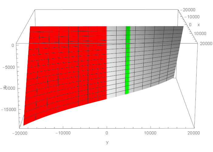
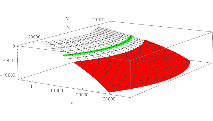
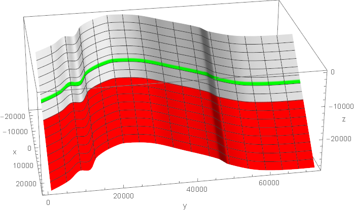
Figure S2. Configuration N1 for the negatively curved surface. This configuration is used for source tests and target tests and is one of the configurations used in the main article. The source region is shown in red, and the target region is shown in green. The target region is a strip one-element thick; the figure assumes an element size of 1200 m. Grid lines are contours of constant depth () and contours of constant distance along strike (), and they do not represent fault elements.
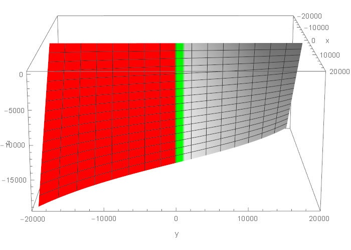
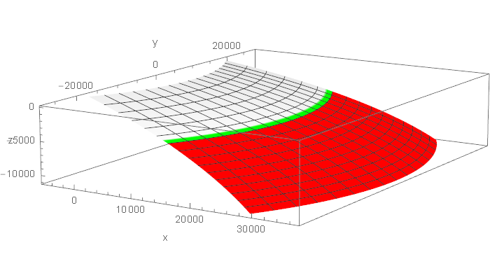
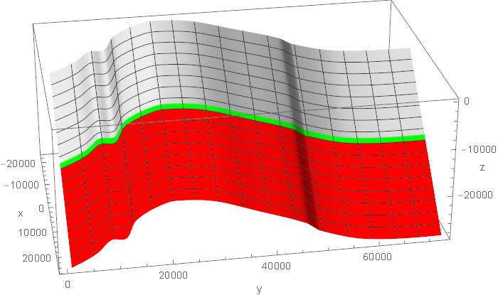
Figure S3. Configuration N2 for the negatively curved surface. This configuration is used for propagation tests and is one of the configurations used in the main article. The source region is shown in red, and the target region is shown in green. The target region is a strip one-element thick; the figure assumes an element size of 1200 m. Grid lines are contours of constant depth () and contours of constant distance along strike (), and they do not represent fault elements.
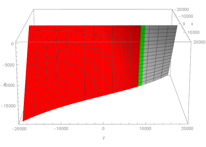
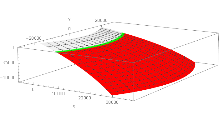
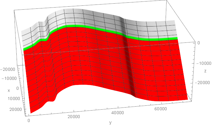
Figure S4. Configuration N3 for the negatively curved surface. This configuration is used for source tests and target tests. The source region is shown in red, and the target region is shown in green. The target region is a strip one-element thick; the figure assumes an element size of 1200 m. Grid lines are contours of constant depth () and contours of constant distance along strike (), and they do not represent fault elements.
Figure S5. Configuration N4 for the negatively curved surface. This configuration is used for propagation tests. The source region is shown in red, and the target region is shown in green. The target region is a strip one-element thick; the figure assumes an element size of 1200 m. Grid lines are contours of constant depth () and contours of constant distance along strike (), and they do not represent fault elements.
Figure S6. Positively curved fault surface. The surface is a section of an ellipsoid. All dimensions are in meters. The fault trace is a curve, for which the strike angle varies from −30° to +30°. Fault dip is 10° at the top center of the fault and 30° at the bottom center of the fault. The fault extends from the Earth’s surface at , to a maximum depth of approximately . This is a dip-slip (thrust) fault. Grid lines are contours of constant depth () and contours of constant distance along strike (), and they do not represent fault elements.
Figure S7. Configuration P1 for the positively curved surface. This configuration is used for source tests and target tests and is one of the configurations used in the main article. The source region is shown in red, and the target region is shown in green. The target region is a strip one-element thick; the figure assumes an element size of 1200 m. Grid lines are contours of constant depth () and contours of constant distance along strike (), and they do not represent fault elements.
Figure S8. Configuration P2 for the positively curved surface. This configuration is used for propagation tests and is one of the configurations used in the main article. The source region is shown in red, and the target region is shown in green. The target region is a strip one-element thick; the figure assumes an element size of 1200 m. Grid lines are contours of constant depth () and contours of constant distance along strike (), and they do not represent fault elements.
Figure S9. Configuration P3 for the positively curved surface. This configuration is used for propagation tests. The source region is shown in red, and the target region is shown in green. The target region is a strip one-element thick; the figure assumes an element size of 1200 m. Grid lines are contours of constant depth () and contours of constant distance along strike (), and they do not represent fault elements.
Figure S10. Zero-curvature fault surface. The surface is a section of a cylinder with irregular cross section. All dimensions are in meters. The fault trace is a curve, which is obtained by interpolating the waypoints for the North Frontal West fault in UCERF3 fault model v.3.2. Fault dip is 49°. The fault extends from the Earth’s surface at , to a maximum depth of approximately . This is a dip-slip (thrust) fault. Grid lines are contours of constant depth () and contours of constant distance along strike (), and they do not represent fault elements.
Figure S11. Configuration C1 for the zero-curvature surface. This configuration is used for source tests and target tests and is one of the configurations used in the main article. The source region is shown in red, and the target region is shown in green. The target region is a strip one-element thick; the figure assumes an element size of 1200 m. Grid lines are contours of constant depth () and contours of constant distance along strike (), and they do not represent fault elements.
Figure S12. Configuration C2 for the zero-curvature surface. This configuration is used for propagation tests and is one of the configurations used in the main article. The source region is shown in red, and the target region is shown in green. The target region is a strip one-element thick; the figure assumes an element size of 1200 m. Grid lines are contours of constant depth () and contours of constant distance along strike (), and they do not represent fault elements.
Figure S13. Configuration C3 for the zero-curvature surface. This configuration is used for propagation tests. The source region is shown in red, and the target region is shown in green. The target region is a strip one-element thick; the figure assumes an element size of 1200 m. Grid lines are contours of constant depth () and contours of constant distance along strike (), and they do not represent fault elements.
Figure S14. Source test results for negatively curved fault surface configuration N1, shear stress. Refer to Table S7 for a list of all results.
Figure S15. Source test results for negatively curved fault surface configuration N1, normal stress. Refer to Table S7 for a list of all results.
Figure S16. Target test results for negatively curved fault surface configuration N1, shear stress. Refer to Table S7 for a list of all results.
Figure S17. Target test results for negatively curved fault surface configuration N1, normal stress. Refer to Table S7 for a list of all results.
Figure S18. Propagation test results for negatively curved fault surface configuration N2, shear stress. Refer to Table S7 for a list of all results.
Figure S19. Propagation test results for negatively curved fault surface configuration N2, normal stress. Refer to Table S7 for a list of all results.
Figure S20. Source test results for negatively curved fault surface configuration N3, shear stress. Refer to Table S7 for a list of all results.
Figure S21. Source test results for negatively curved fault surface configuration N3, normal stress. Refer to Table S7 for a list of all results.
Figure S22. Target test results for negatively curved fault surface configuration N3, shear stress. Refer to Table S7 for a list of all results.
Figure S23. Target test results for negatively curved fault surface configuration N3, normal stress. Refer to Table S7 for a list of all results.
Figure S24. Propagation test results for negatively curved fault surface configuration N4, shear stress. Refer to Table S7 for a list of all results.
Figure S25. Propagation test results for negatively curved fault surface configuration N4, normal stress. Refer to Table S7 for a list of all results.
Figure S26. Source test results for positively curved fault surface configuration P1, shear stress. The green curve is hard to see because it lies underneath the red curve. Refer to Table S7 for a list of all results.
Figure S27. Source test results for positively curved fault surface configuration P1, normal stress. The green curve is hard to see because it lies underneath the red curve. Refer to Table S7 for a list of all results.
Figure S28. Target test results for positively curved fault surface configuration P1, shear stress. The green curve is hard to see because it lies underneath the red curve. Refer to Table S7 for a list of all results.
Figure S29. Target test results for positively curved fault surface configuration P1, normal stress. The green curve is hard to see because it lies underneath the red curve. Refer to Table S7 for a list of all results.
Figure S30. Propagation test results for positively curved fault surface configuration P2, shear stress. The green curve is hard to see because it lies underneath the red curve. Refer to Table S7 for a list of all results.
Figure S31. Propagation test results for positively curved fault surface configuration P2, normal stress. The green curve is hard to see because it lies underneath the red curve. Refer to Table S7 for a list of all results.
Figure S32. Propagation test results for positively curved fault surface configuration P3, shear stress. The green curve is hard to see because it lies underneath the red curve. Refer to Table S7 for a list of all results.
Figure S33. Propagation test results for positively curved fault surface configuration P3, normal stress. The green curve is hard to see because it lies underneath the red curve. Refer to Table S7 for a list of all results.
Figure S34. Source test results for zero-curvature fault surface configuration C1, shear stress. The green curve is hard to see because it lies underneath the red curve. Refer to Table S7 for a list of all results.
Figure S35. Source test results for zero-curvature fault surface configuration C1, normal stress. The green curve is hard to see because it lies underneath the red curve. Refer to Table S7 for a list of all results.
Figure S36. Target test results for zero-curvature fault surface configuration C1, shear stress. The green curve is hard to see because it lies underneath the red curve. Refer to Table S7 for a list of all results.
Figure S37. Target test results for zero-curvature fault surface configuration C1, normal stress. The green curve is hard to see because it lies underneath the red curve. Refer to Table S7 for a list of all results.
Figure S38. Propagation test results for zero-curvature fault surface configuration C2, shear stress. Refer to Table S7 for a list of all results.
Figure S39. Propagation test results for zero-curvature fault surface configuration C2, normal stress. Refer to Table S7 for a list of all results.
Figure S40. Propagation test results for zero-curvature fault surface configuration C3, shear stress. Refer to Table S7 for a list of all results.
Figure S41. Propagation test results for zero-curvature fault surface configuration C3, normal stress. Refer to Table S7 for a list of all results.
Download: NFW_UCERF3_FM3_2.zip [Zipped Text file; ~4 KB] An excerpt from UCERF3 fault model v.3.2, which defines the geometry of the North Frontal West fault.
Download: NFW_Interpolated.zip [Zipped Text file; ~136 KB] Data file that contains the fault trace () coordinates and rake angles, tabulated as functions of distance along strike, for our zero-curvature (cylindrical) fault surface. Function values are given at intervals of 10 m. The file format is documented by comments at the start of the file.
[ Back ]