This electronic supplement contains a description of the operations involved in the automated receiver function (RF) workflow, a table showing the number of events used in each RF workflow and event overlap, and figures of event magnitude distributions and resulting RFs.
In this section, we provide a step-by-step description of the operations involved in our automated RF workflow. The objective is to complement the more cursory overview given in the main article.
(a) Earthquake list: Compile a list of all earthquakes with magnitude mb ≥5.5 that have occurred since 1 January 1980. This is done through the Incorporated Research Institutions for Seismology Data Management Center (IRIS-DMC) Web Services with the FetchEvent script (see Data and Resources).
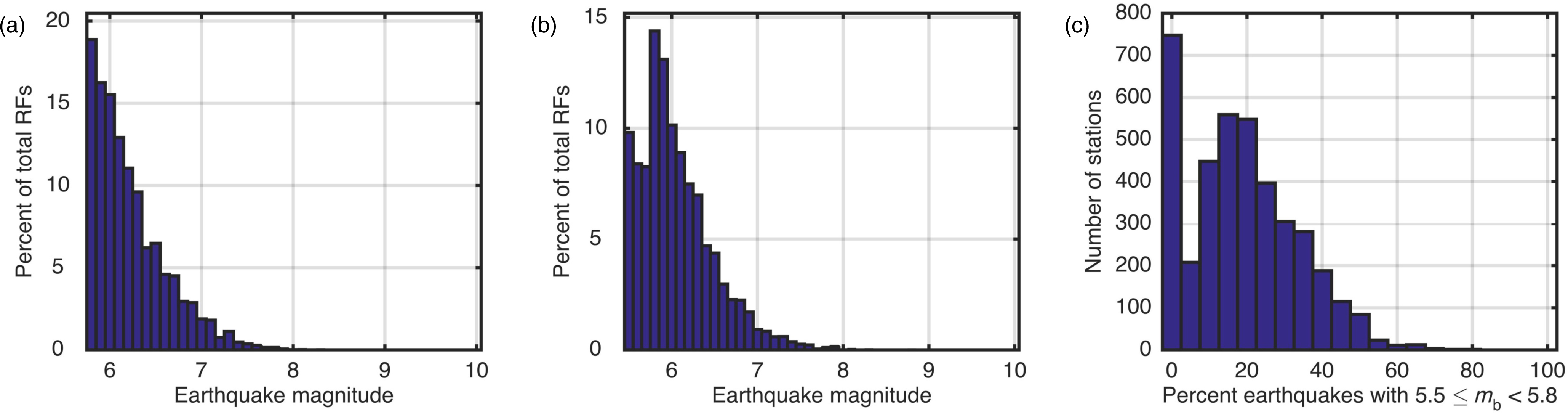
(b) Preliminary earthquake selection: For each station, identify earthquakes that occur while the station is in operation and that fall within the 29°–98° epicentral distance range. The epicentral distance condition prevents the inclusion of P waves that are triplicated at the mantle transition zone (<29°) or diffracted at the core–mantle boundary (>98°). Different magnitude criteria are applied depending on whether the stations are permanent or temporary (see Fig. S1 for magnitude distributions). For permanent stations, retain only events with magnitude mb ≥5.8, because we assume there are enough of these to yield comprehensive ray parameter/back-azimuthal coverage. For temporary stations, retain events with magnitude mb ≥5.5. Although records from events in the 5.5–5.7 magnitude range tend to be noisier than those from larger magnitude earthquakes, they may still contribute constructively to signals of interest while filling gaps in ray parameter and back-azimuthal coverage (see Fig. S2).
(c) Data download: Download data through the IRIS-DMC Web Services using the FetchData script (see Data and Resources). For each station and event selected in (b), download three-component seismic traces that start 30 s prior to the theoretical arrival of the P wave and have a total duration of 150 s. Both BH and HH channels are downloaded.
(d) Data preprocessing: The downloaded seismic traces are first analyzed for consistency with respect to the parameters of the requests (start time, length, etc.). The traces are then tapered with a 7.5 s Hamming taper, filtered with a zero-phase Butterworth band-pass filter (cutoffs at 0.03 and 4.9 Hz), and downsampled to 10 Hz. Last, they are rotated to the vertical–radial–transverse (Z–R–T) coordinate system and filed according to data and event information. The horizontal slowness of the primary incident teleseismic wave is estimated for each station–event pair using travel-time tables computed with the iaspei-tau package for a standard 1D global model (see Snoke, 2009; see also Data and Resources).
(e) Quality control: A second round of data selection based on the signal-to-noise ratio (SNR) of the incident and converted waves occurs here. For both radial and vertical traces, the noise is computed over a window extending between 7.5 and 25 s, whereas the signal is computed over two windows, one that includes the main pulse of the incident wave (30–37.5 s) and another that samples the coda (45–52.5s). We only retain signals that have an SNR of 8.75 and 10 dB for the incident wave on the R and Z components, respectively, and a net SNR decay between the incident wave and its coda. This selection procedure is repeated in three frequency bands, 0.03–1.5 Hz, 0.1–1.5 Hz, and 0.5–1.5 Hz, to retain desirable signals that may be confined to limited bandwidths. These selection criteria are more restrictive on noisier signals from moderate magnitude events (5.5 ≤ mb < 5.8) than on signals from larger magnitude sources (mb ≥5.8; see Fig. S1).
(f) Analysis: For all selected traces, calculate the polarization of the incident wave by singular value decomposition (SVD) on the radial and transverse components and use this information to estimate the average P-wave velocity beneath each station. Estimate the S-wave velocity using the approach described in Bostock and Rondenay (1999), which is based on the free-surface transfer matrix of Kennett (1991). Use the polarization information to rotate all traces into the L–Q–T coordinate system. Deconvolve the L component from the Q and T components to obtain the so-called radial and transverse RFs. The resulting RFs distributed at the time of publication were obtained by spectral division with an objective regularization parameter based on pre-event noise.
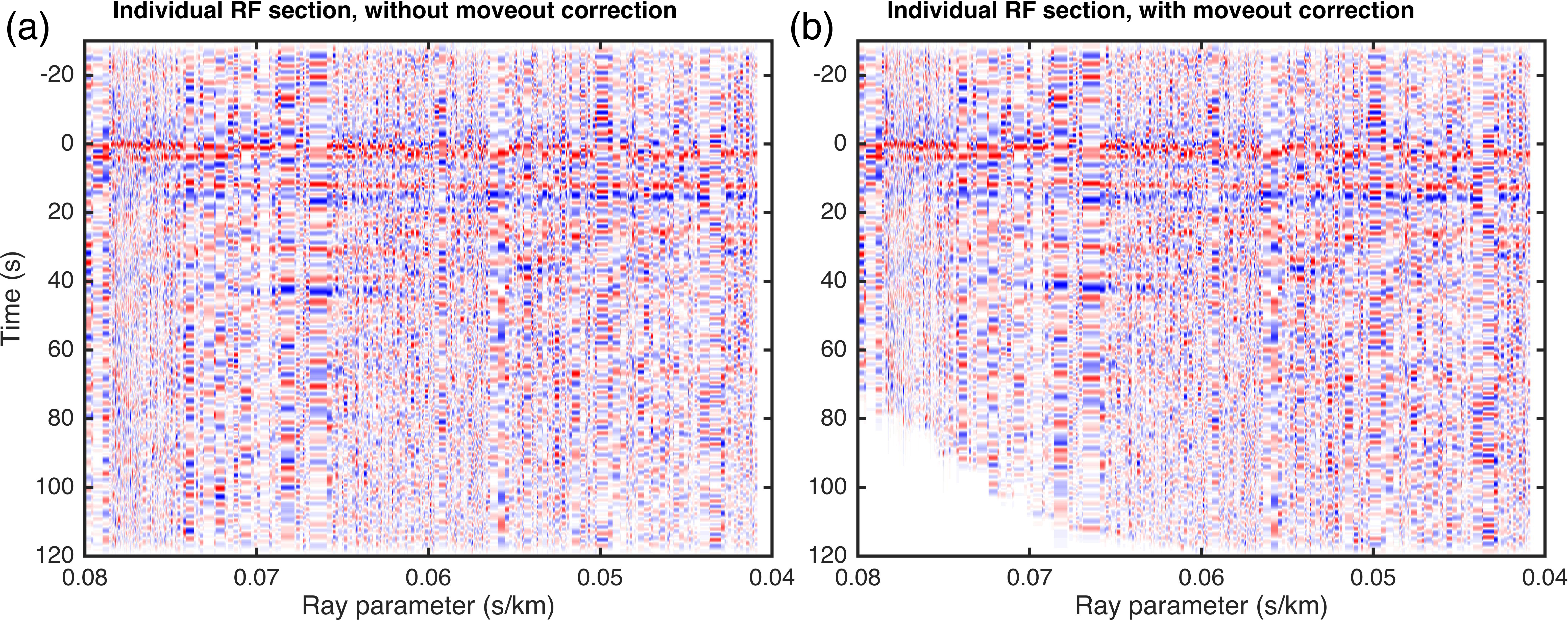
(g) Postprocessing: Apply moveout correction to the RFs. Taper the RFs with a 5 s cosine taper applied to both ends of the time series. Filter with a zero-phase Butterworth band-pass filter with cutoffs at 0.05 and 1.5 Hz for 0–200 km stacks/sections focusing on the lithosphere and at 0.05 and 0.5 Hz for 0–800 km stacks/sections focusing on the mantle transition zone. The RFs are then mapped to depth and either stacked or displayed as sections as described in the main article. Full-length RFs for station IU-HRV are shown in Figure S3, with and without moveout correction.
We now put our results to the test by comparing them with RFs from another automated database, the Earthscope Automated Receiver Services (EARS), and RFs that are generated with extensive user input (referred to as manual RFs). Below, we first briefly describe the EARS and manual RF workflows, and then compare the approaches for a set of representative individual stations and across regional networks.
The automated processing done by EARS is described in Crotwell and Owens (2005). The RFs are computed by deconvolving the vertical component from the radial and transverse components using the time-domain iterative approach of Ligorría and Ammon (1999). The signals are filtered with a low-pass Gaussian filter of 2.5 Hz width (i.e., ∼0.45 s standard deviation), yielding RFs that are dominated by lower frequencies than those generated in Global Lithospheric Imaging with Earthquake Recordings (GLImER). The EARS workflow then stacks the direct Ps Moho arrivals with their corresponding Pps and Pss free-surface multiples (H-K staking method of Zhu and Kanamori, 2000) to estimate the VP/VS ratio of the crust and Moho depth beneath each station. RFs are retained based on how robust their stack is and, ultimately, how well they match the preferred Moho depth and VP/VS ratio.
To generate manual RFs, we visually select input R–T–Z traces that exhibit high SNR in three frequency bands (0.03–4.9 Hz, 0.1–4.9 Hz, and 0.5–4.9 Hz), carry out the deconvolution, and visually inspect the resulting RFs for further selection of stable signals (i.e., signals that do not exhibit strong oscillations and/or apparent signals prior to zero time). For permanent stations like IU-HRV, for which traces from 1781 events were initially downloaded, this manual processing takes, on average, 2–3 hrs, in stark contrast to ∼1–2 min run time for the GLImER automated workflow.
We compare the results from the three RF workflows on three individual stations that represent various settings encountered across the entire database. Station IU-HRV is a permanent station that has been in operation for nearly 30 years. It is located in Harvard, Massachusetts, and the seismometer rests directly on bedrock. As such, it represents what one may consider an ideal station. Stations TA-L49A and TA-R53A are temporary stations of the Earthscope Transportable Array that were each in operation for ∼22 months. TA-L49A is located in Milan, Michigan, on the southeastern edge of the Michigan basin, and sits on top of an ∼1-km-thick sedimentary layer (see e.g., Howell and van der Pluijm, 1999). This station is expected to produce lower quality results compared to IU-HRV because of the shorter recording time (meaning worse event coverage) and the fact that it sits on sediments. TA-R53A is located in Hurricane, West Virginia, in the middle of the Appalachian basin, sitting on top of an ∼5-km-thick sedimentary layer (see, e.g., Howell and van der Pluijm, 1999). This is deemed a problematic station where we expect the RFs to be completely dominated by multiples in the thick sedimentary layer.
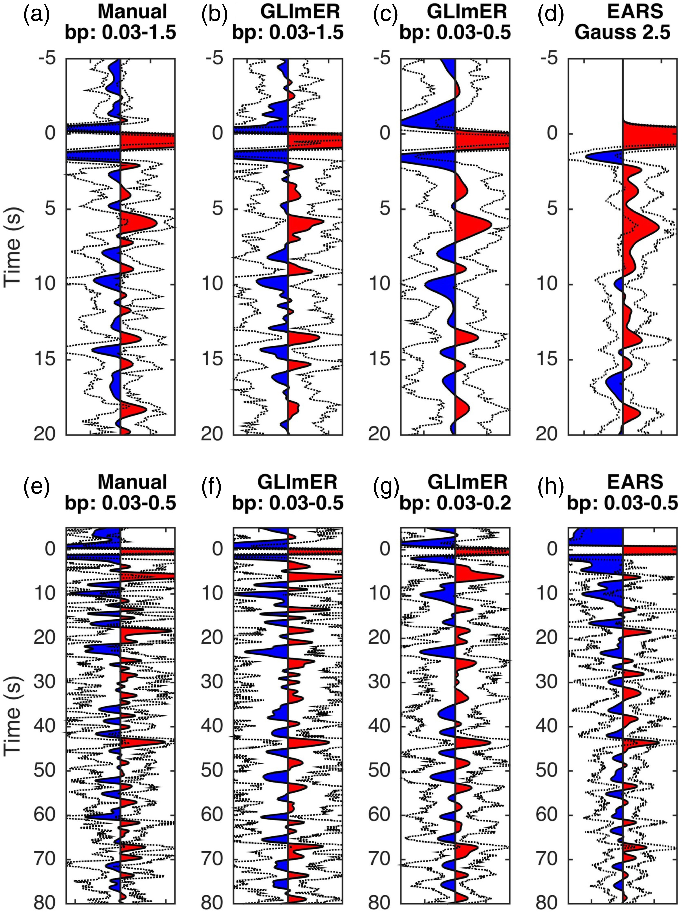
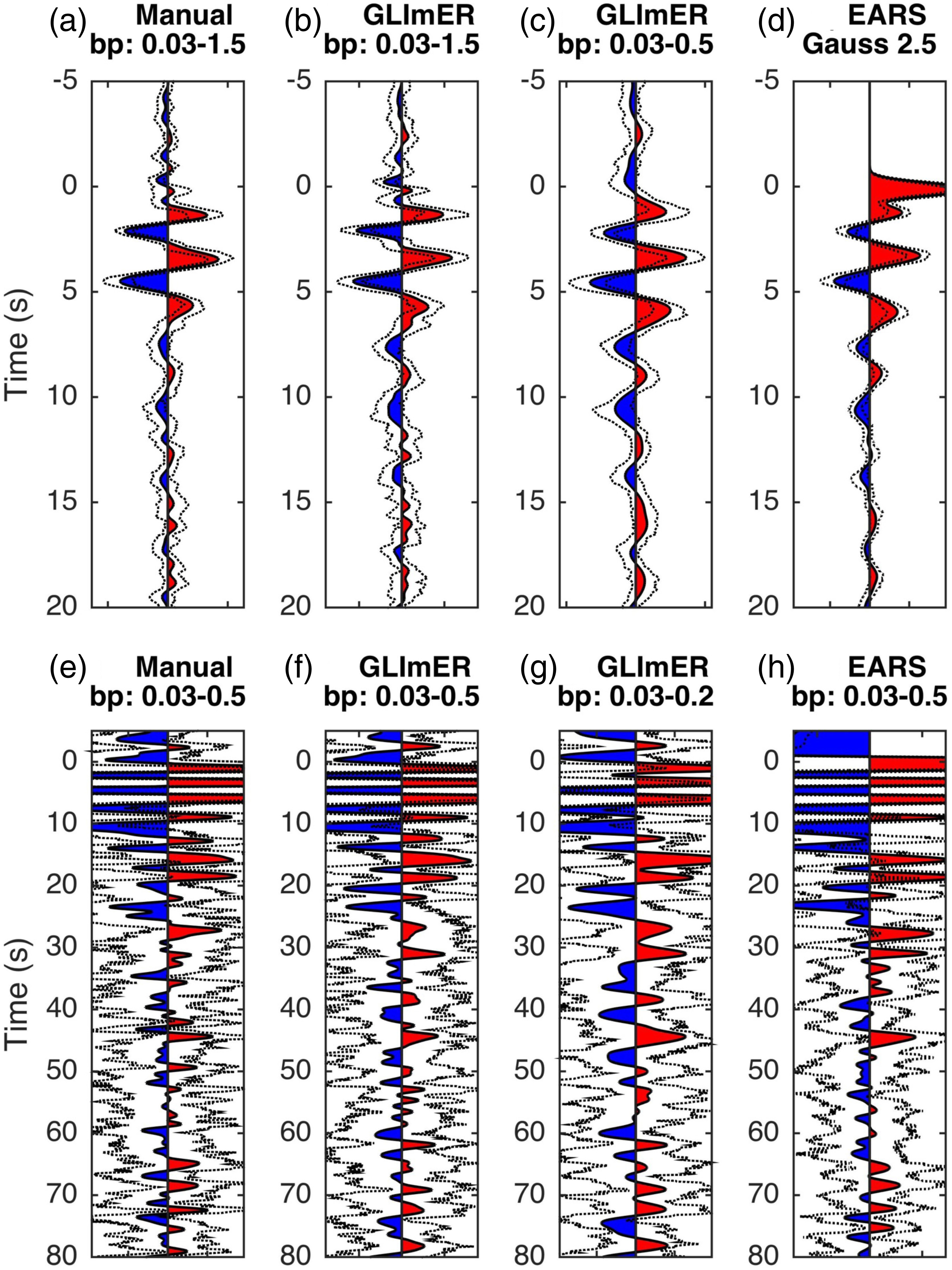
The comparisons between the different RFs at stations IU-HRV, TA-L49A, and TA-R53A are shown in Figures S4, S5, and S6, respectively. When comparing the various waveforms, one must take into account the fact that the EARS RFs are computed with the Z–R components, which introduces a large peak at 0 s (i.e., the incident wave on the R component deconvolved by itself) that is not present in the L–Q RFs computed either for GLImER or manually. One should also note that the EARS RFs are filtered with a more aggressive low-pass filter than those in GLImER. Therefore, to assist in the comparison with EARS, we also show a version of the GLImER stacked RFs filtered with a low cutoff of 0.5 Hz (instead of the 1.5 Hz cutoff used for our 0–20 s/0–200 km RFs).
Table S1 shows the total number of event recordings downloaded for GLImER at the three stations and contrasts the number of events retained in each workflow. For IU-HRV, the number of retained events decreases significantly from GLImER to manual to EARS. This is a pattern observed in many other permanent stations globally when comparing GLImER and EARS (e.g., 1500 events for GLImER versus 200 events for EARS at station II-RAYN in Saudi Arabia). It is a consequence of the two automated workflows selecting vastly different numbers of earthquakes at the outset. The smaller sample sizes of the manual and EARS workflows do not overlap completely with the more comprehensive sample used for GLImER. This also reflects the difference in selection criteria between the various workflows. For temporary stations, all three workflows retain roughly the same number of events; the initial selection by the two automated workflows returns similar numbers of events here, in contrast to the permanent station.
Regardless of the final earthquake selection, the RFs generated by the various workflows are generally similar in their first-order features (see Figs. S4–S6). As expected, the RFs from IU-HRV provide the clearest image of subsurface structure. We detect pulses corresponding to the Moho, mid-lithosphere discontinuity (MLD), lithosphere–asthenosphere boundary (LAB), and mantle transition zone discontinuities in all the stacked RFs (see main article for further discussion). At TA-L49A, the first few seconds of the RF are dominated by a set of large pulses related to the thin sedimentary layer, but the rest of the record is more stable and allows the identification of a clear Moho signal at ∼6 s, and mantle transition zone discontinuities at ∼44 and 67 s. At TA-R53A, the RFs are dominated by strong multiples from the thick sedimentary layer to at least 30 s. There appears to be a signal corresponding to the 410 km discontinuity at ∼45 s, but nothing clear for the 660 km discontinuity.
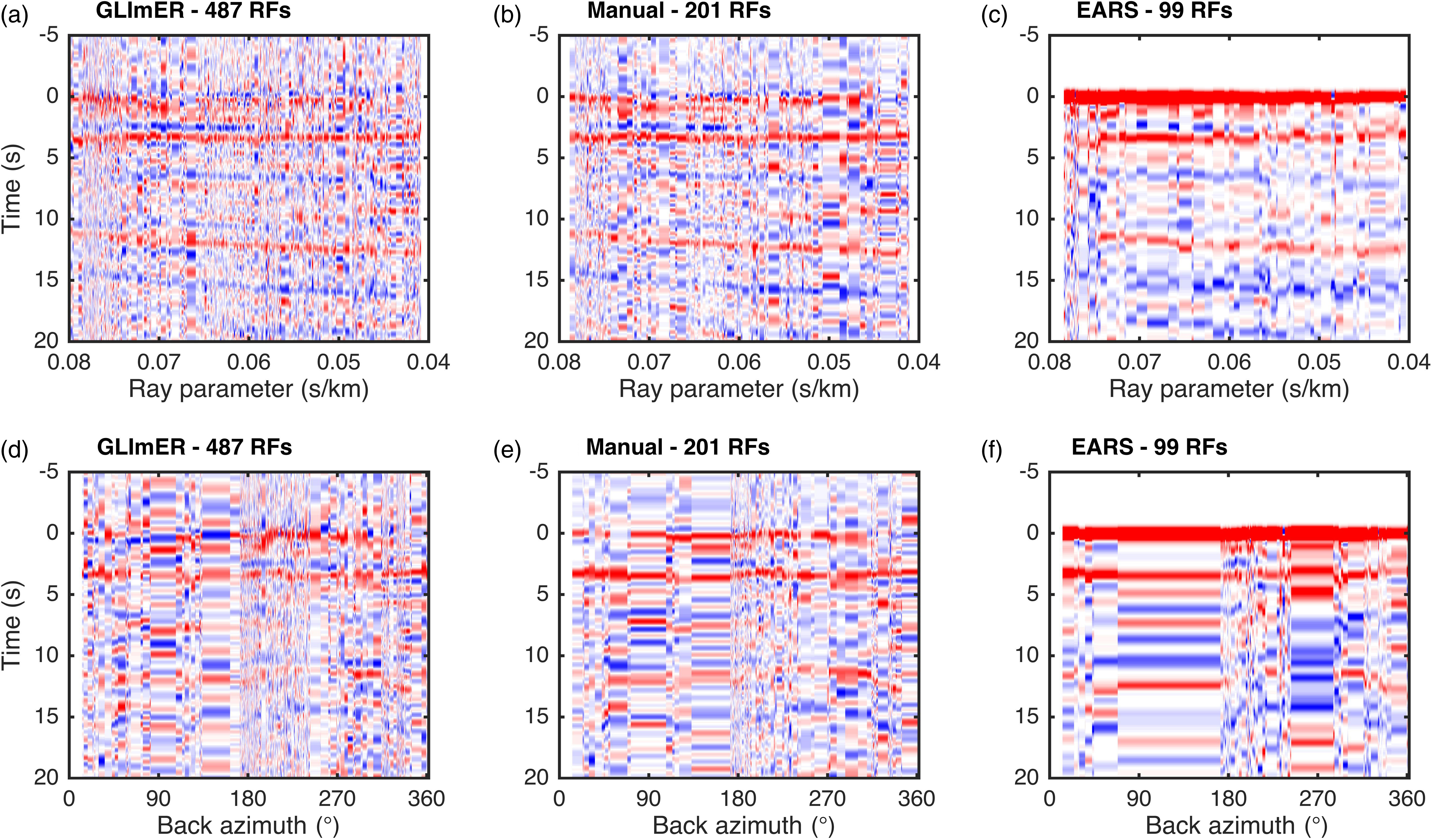
Owing to stricter selection criteria at IU-HRV and other permanent stations, the scatter of the RFs (expressed as the interquartile range in Figs. S4–S6) appears generally smaller for the EARS workflow than for the GLImER and manual workflows. However, it is clear from sections of individual RFs (see Fig. S7 for sections at IU-HRV) that most of the RFs retained in the latter two contribute constructively to the signals in the stack. As a consequence, the GLImER and manual RFs tend to exhibit stronger signals associated with smaller sub-Moho discontinuities such as the MLD and LAB. Furthermore, the GLImER RFs afford better coverage in terms of ray parameter (epicentral distance) and back azimuth than the two other workflows (see e.g., Fig. S7), making them more suitable for anisotropy analyses or migration imaging approaches.
Finally, we propose to investigate how the two automated workflows—GLImER and EARS—compare when it comes to characterizing specific structures across the large distances covered by regional and continental-sized networks. A perfect setting for such a comparison is the continental United States, which with the Earthscope project and numerous Program for the Array Seismic Studies of the Continental Lithosphere (PASSCAL) deployments, has now been sampled with unprecedented spatial density.
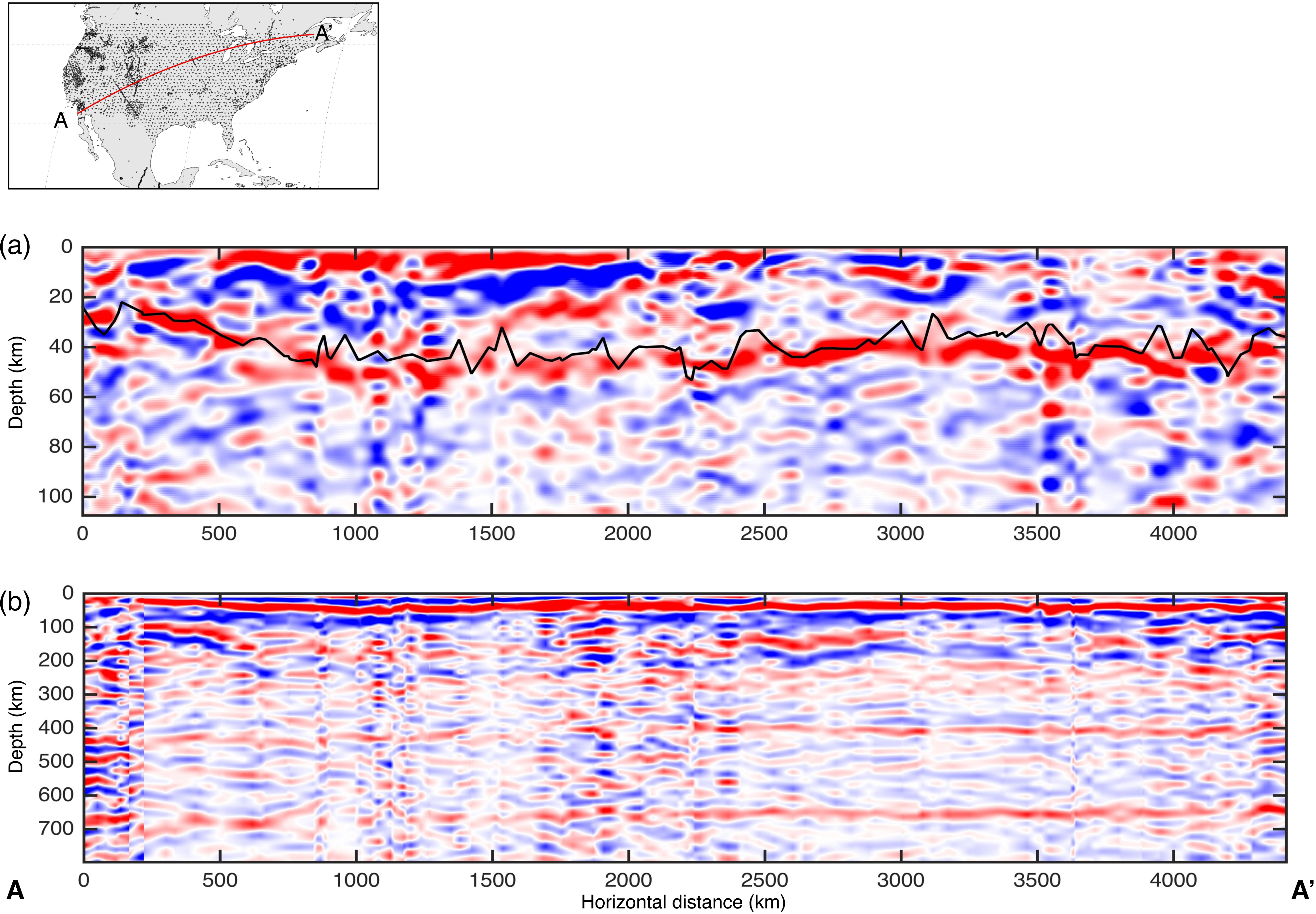
Following the simplest 2D imaging technique described in the main article, which consists of juxtaposing RFs, we use the GLImER RFs to generate a long-range profile extending from southeastern California to northeastern Maine (Fig. S8). The profile is shown over two depth ranges: (1) 0–105 km depth, to focus on crustal and uppermost mantle structure, and (2) 0–800 km depth, to emphasize mantle transition zone structures. The first profile gives a clear picture of the Moho, which is seen as a strong positive (red) signal across the entire section. The second, deeper, profile exhibits strong positive (red) signals corresponding to phase transitions at depths of ∼410 and ∼660 km. As discussed in the main article, our simple imaging technique precludes an accurate representation of deep discontinuities due to extensive horizontal averaging and the use of a uniform 1D model to transform conversion times into depth.
To compare our results with those from EARS, we plot Moho depth estimates produced by EARS on top of our shallower profile (Fig. S8a). The general trend of the Moho across the continent is well correlated between the two methods. However, at smaller scales, EARS exhibits some rapid variations in Moho depth, which are not evident in the long-range profile from GLImER. This may be due to a discrepancy in lateral resolution between the two methods or perhaps, in some cases, to a misidentification of the Moho signal by the H-K stacking approach used by EARS (e.g., at x = 1500 km and at x = 3000–3100 km). This is not to say that one of the databases is superior to the other. As discussed at the beginning of the main article, the two databases serve different purposes and should be seen as complementary products. One of the central goals of EARS is to provide estimates of Moho depth and crustal VP/VS beneath each station. GLImER, on the other hand, is intended as a more general imaging tool for all discontinuities with the crust and upper mantle.
Table S1. Number of events used in each RF workflow and event overlap.
Figure S1. Distribution of magnitudes for events used in the GLImER database of automated RFs. Distributions are given for (a) permanent stations, where mb ≥5.8 and (b) temporary stations, where mb ≥5.5. (c) Number of temporary stations as a function of the percentage of selected earthquakes that fall in the magnitude range 5.5 ≤ mb < 5.8. As seen in (a), selected earthquakes with mb ≥5.8, follow a power-law distribution, suggesting that the selection criteria operate relatively evenly over these magnitude events. At temporary stations, the selection criteria reject more events in the 5.5 ≤ mb < 5.8 range than in the mb ≥5.8 range, as seen in (b), because weaker events tend to generate noisier signals. Events in the 5.5 ≤ mb < 5.8 range represent on average ∼27% of events used at temporary stations, as seen in (c).
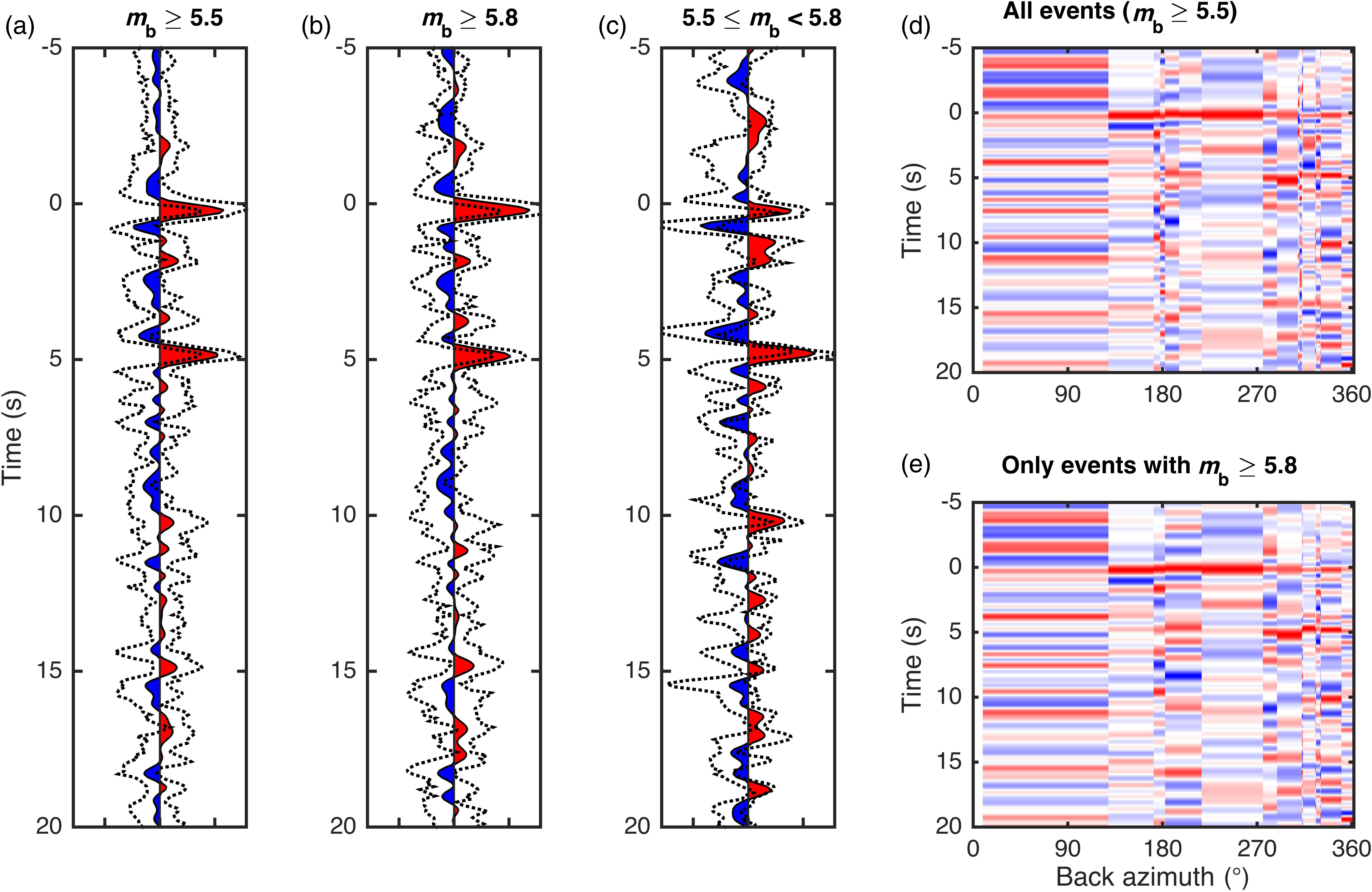
Figure S2. Contribution of lower-magnitude events to RFs at temporary stations. Illustration with an example from station XB96-VSGL, situated in the southeast Canadian shield. (a–c) Stacked RFs using (a) all selected events with mb ≥5.5, a total of 22 events, (b) larger earthquakes with mb ≥5.8, a total of 14 events, and (c) only smaller earthquakes with 5.5 ≤ mb < 5.8, a total of 8 events. The variability of the individual traces used in the stacks is expressed via the interquartile range, shown as dotted black lines in (a–c). (d,e) Individual RF sections for (d) events with mb ≥5.5, and (e) events with mb ≥5.8. Despite exhibiting higher variability, smaller earthquakes with magnitudes in the 5.5 ≤ mb < 5.8 range contribute constructively to first-order signals appearing in the final stack (e.g., the Moho at ∼5 s) and yield a more comprehensive back-azimuthal coverage [notably in the vicinity of 180° and 300°; compare (d) and (e)].
Figure S3. Sections showing full-length individual RFs as a function of ray parameter for station IU-HRV. RFs are shown (a) without moveout correction, and (b) with moveout correction. The moveout correction is applied to take into account varying incidence angles as a function of ray parameter (see, e.g., Rondenay, 2009). Stacked RFs shown in the main article are obtained by summing the traces in (b), converting times into depths, and cutting widows between 0 and 200 km (∼0–20 s) and 0–800 km (∼0–78 s).
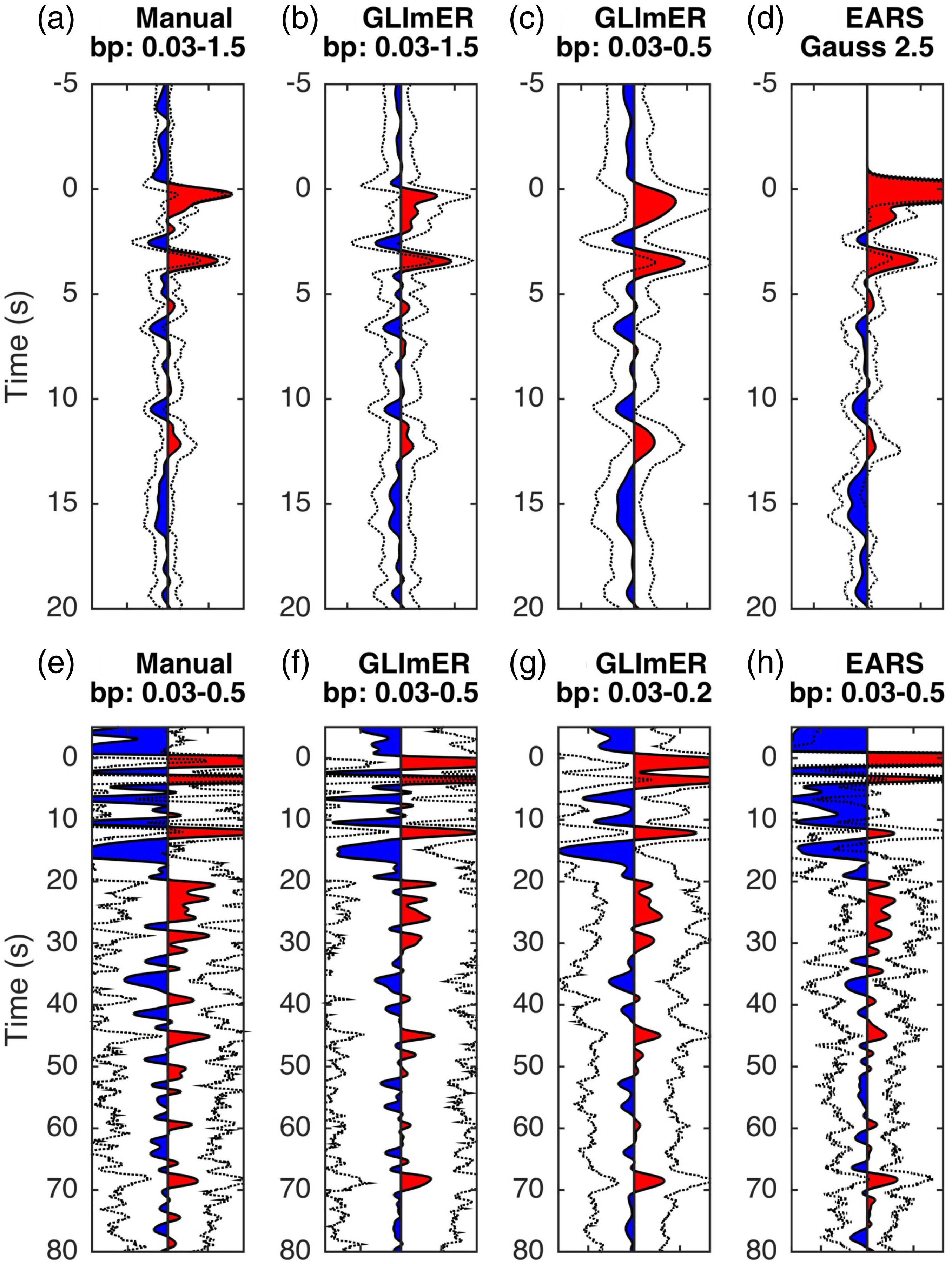
Figure S4. Comparison between manual, GLImER, and EARS RFs for permanent station IU-HRV. The station is located in Harvard, Massachusetts, and sits directly on bedrock. (a–h) The stacked RFs over two different time windows (−5 to 20 s and −5 to 80 s) for the various workflows and filter parameters indicated in the labels. The variability of the individual traces used in the stacks is expressed via the interquartile range, shown as dotted black lines in (a–c).
Figure S5. Comparison between manual, GLImER, and EARS RFs for temporary station TA-L49A. The station is located in Milan, Michigan, and sits on ∼1 km of sediments. (a–h) The stacked RFs over two different time windows (−5 to 20 s and −5 to 80 s) for the various workflows and filter parameters indicated in the labels. The variability of the individual traces used in the stacks is expressed via the interquartile range, shown as dotted black lines in (a–c).
Figure S6. Comparison between manual, GLImER, and EARS RFs for temporary station TA-R53A. The station is located in Hurricane, West Virginia, and sits on ∼5 km of sediments. (a–h) The stacked RFs over two different time windows (−5 to 20 s and −5 to 80 s) for the various workflows and filter parameters indicated in the labels. The variability of the individual traces used in the stacks is expressed via the interquartile range, shown as dotted black lines in (a–c).
Figure S7. Comparison of individual RF sections generated by manual, GLImER, and EARS workflows for permanent station IU-HRV. Top and bottom rows show RF coverage as a function of ray parameter (inversely proportional to epicentral distance) and back azimuth, respectively. The title of each panel indicates the type of workflow followed by the total number of resulting RFs. Note that the GLImER workflow yields a significantly more comprehensive coverage in terms of both ray parameter and back azimuth than the other workflows.
Figure S8. Comparison of long-range RF profiles across regional networks generated by GLImER and EARS workflows. The profiles extend across the United States from southwestern California to northeastern Maine, following the red line labeled A–Aʹ on the map. (a) Focuses on crustal and upper-mantle structure and provides a direct comparison between the GLImER-based image of the Moho (prominent red signal between ∼25 and 50 km depth) and the Moho depth estimates from EARS (thick black line). (b) Focuses on mantle transition zone discontinuities observed at ∼410 and ∼660 km depth across the entire section. Sections are generated by simple juxtaposition of individual RFs, interpolation onto a regular grid, and application of a spatial Gaussian filter (horizontal, 12 km standard deviation).
The data analyzed to date as part of this project were downloaded using the web services of the Incorporated Research Institutions for Seismology Data Management Center (IRIS-DMC; https://service.iris.edu, last accessed November 2016). Travel-time tables computed with the iaspei-tau package can be found at https://seiscode.iris.washington.edu/projects/iaspei-tau (last accessed November 2016). The Global Lithospheric Imaging with Earthquake Recordings (GLImER) webpage and its map can be found at http://stephanerondenay.com/glimer-web.html (last accessed November 2016) and http://stephanerondenay.com/glimermap (last accessed November 2016), respectively.
Bostock, M. G., and S. Rondenay (1999). Migration of scattered teleseismic body waves, Geophys. J. Int. 137, 732–746.
Crotwell, H. P., and T. J. Owens (2005). Automated receiver function processing, Seismol. Res. Lett. 76, no. 6, 702–709.
Howell, P. D., and B. A. van der Pluijm (1999). Structural sequences and styles of subsidence in the Michigan basin, Geol. Soc. Am. Bull. 111, no. 7, 974–991.
Kennett, B. L. N. (1991). The removal of free surface interactions from three-component seismograms, Geophys. J. Int. 104, 153–163.
Ligorría, J. P., and C. J. Ammon (1999). Iterative deconvolution and receiver-function estimation, Bull. Seismol. Soc. Am. 89, no. 5, 1395–1400.
Rondenay, S. (2009). Upper mantle imaging with array recordings of converted and scattered teleseismic waves, Surv. Geophys. 30, 377–405, doi: 10.1007/s10712-009-9071-5.
Snoke, J. A. (2009). Traveltime Tables for iasp91 and ak135, Seismol. Res. Lett. 80, no. 2, 260–262.
Zhu, L., and H. Kanamori (2000). Moho depth variation in southern California from teleseismic receiver functions, J. Geophys. Res. 105, 2969–2980.
[ Back ]