The electronic supplement includes:
Table S1. HASH parameter settings.
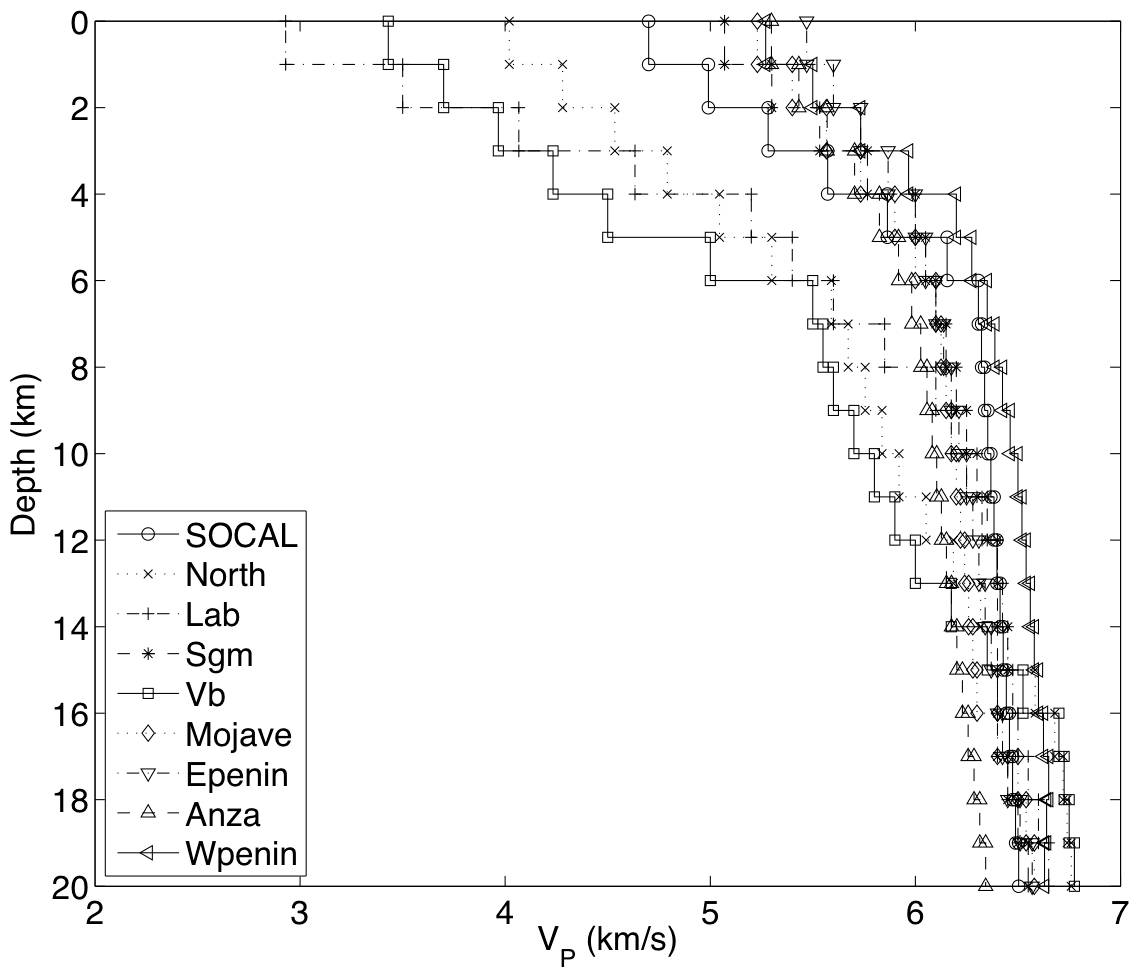
We use nine different 1D velocity models for southern California region (Figure S1) to account for regional variations in the velocity structure. The SOCAL model is a smoothed version of a standard 1D model for southern California (Shearer, 1997). The other eight 1D models are the averages of the 3D velocity model of Hauksson (2000) in different regions of southern California. Among them, the North model is for the vicinity of Northridge, the Lab model is for the Los Angeles basin, the Sgm model is for the San Gabriel Mountains, the Vb model is for the Ventura Basin, the Mojave model is for the Mojave Desert, the Epenin model is for the east Peninsular Range, the Wpenin model is for the west Peninsular Range, and the Anza model is for the Anza area.
Figure S1. Nine 1D velocity models for the southern California region used in the HASH program.
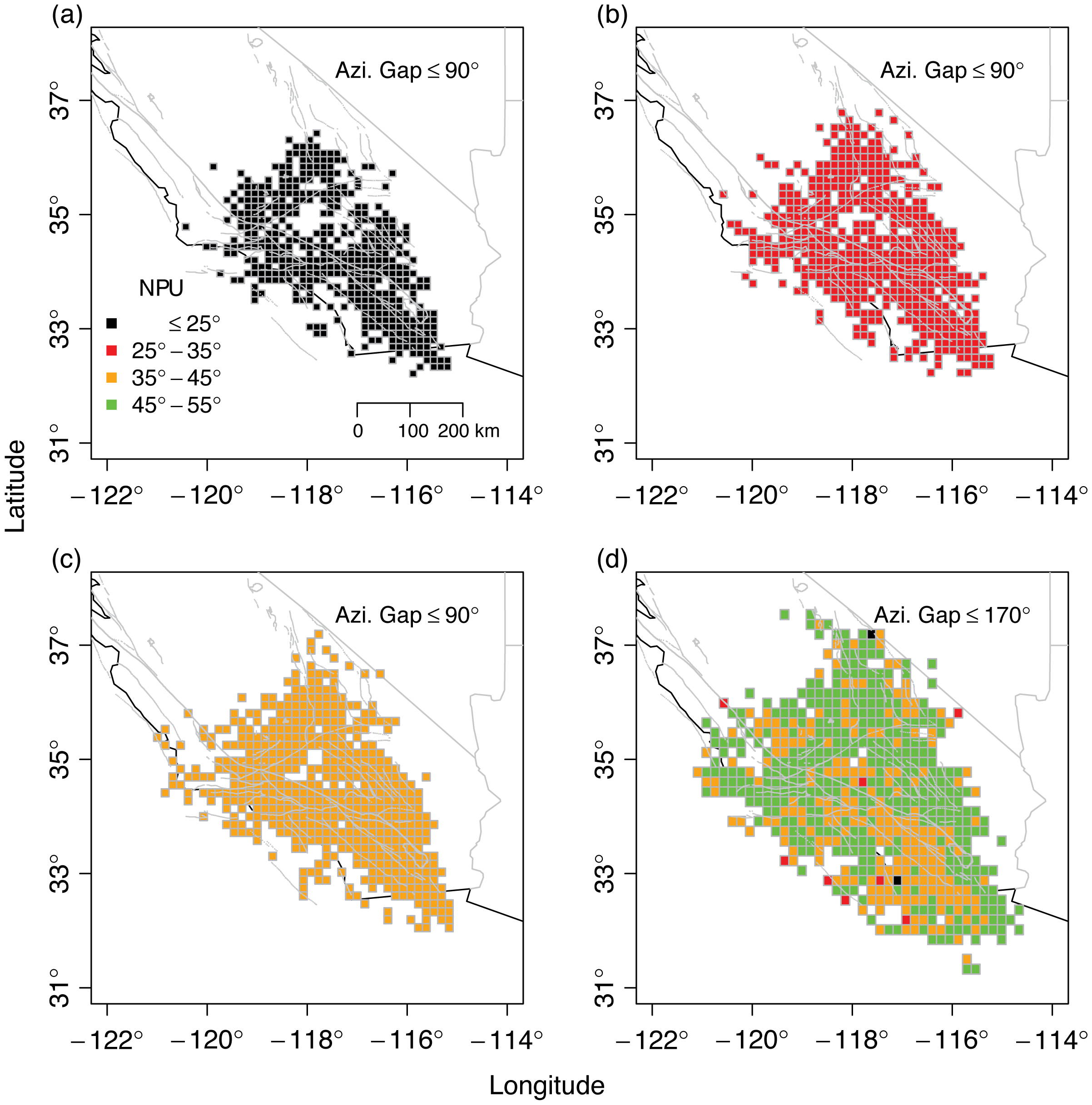
Figure S2 shows the geographical distribution of earthquakes with focal mechanism quality A, B, C, and D and associated mean nodal plane uncertainty. As quality downgrades from A to D, the geographical coverage of data extends across the southern California. For focal mechanisms with quality D, there are some grids with small mean nodal plane uncertainties although the azimuthal gap may be large. Focal mechanisms of all qualities are present in the Los Angles basin, the San Bernardino area, the east California shear zone, the Elsinore faults zone and the San Jacinto faults zone.
Figure S2. The geographical coverage of quality A (a), B (b), C (c) and D (d) focal mechanisms in southern California. Earthquakes of each quality are subdivided into each 20 × 20 km2 grid, and each grid is colored by the mean of nodal plane uncertainties (NPU) inside with color legend in (a). The azimuthal gap for each quality is labeled in the top right corner in each subplot.
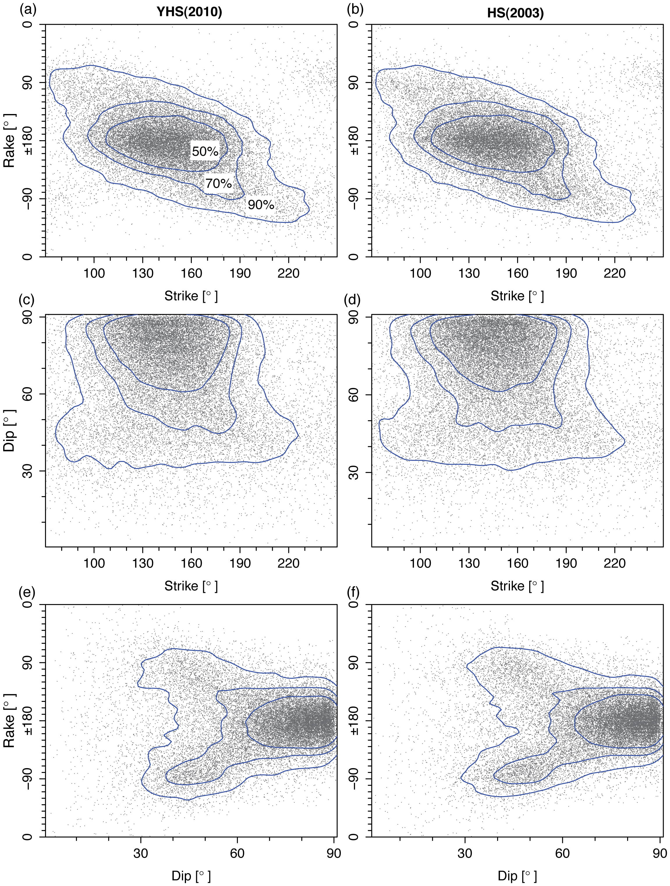
Figure S3. A parallel comparison of 23,420 common earthquakes in the YHS2010 catalog (left column) and the HS2003 catalogs (right column) (Hardebeck and Shearer, 2003) for focal mechanism parameters. The contour lines represent the 90%, 70% and 50% data kernel density distribution from outer to inner.
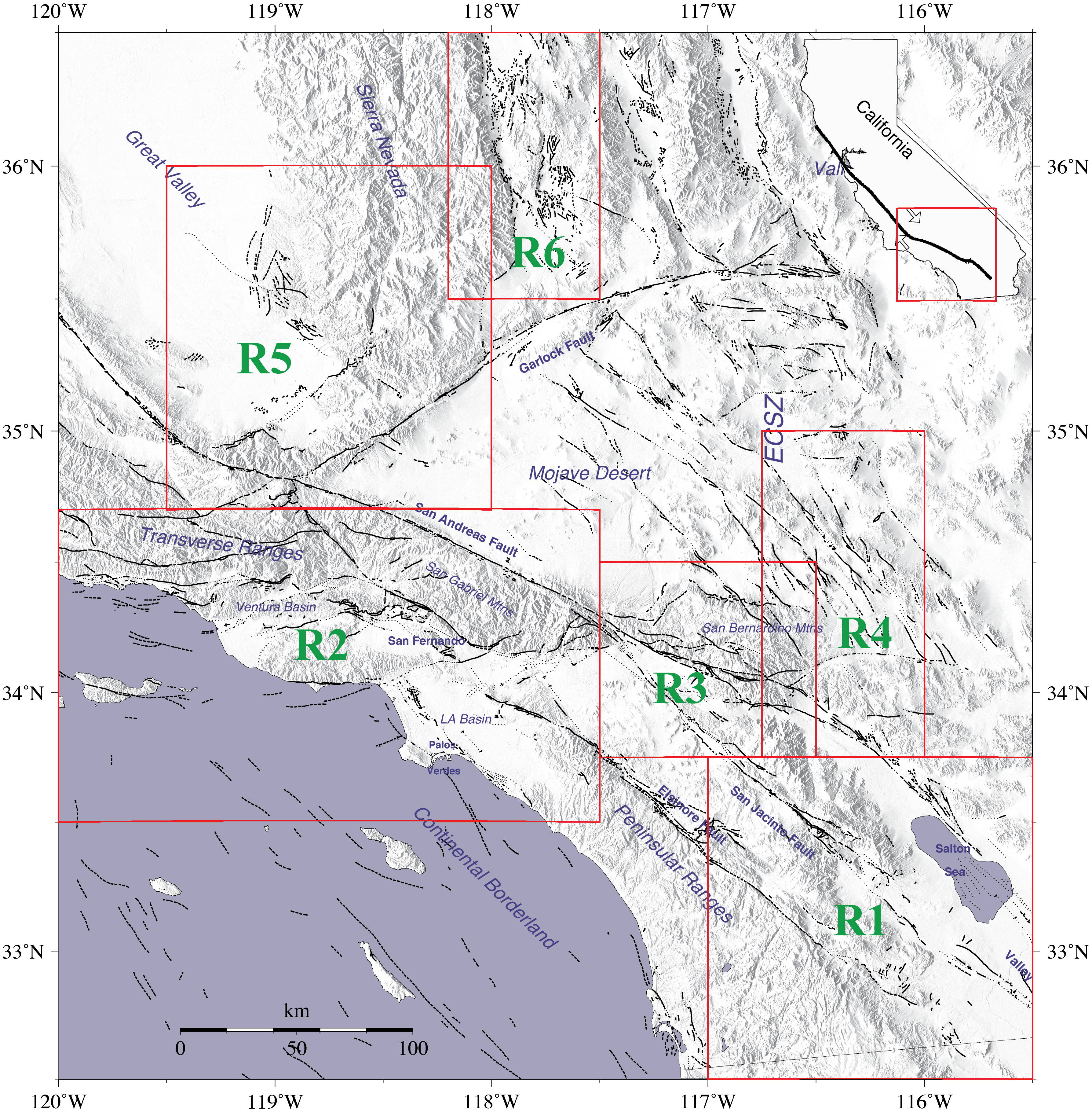
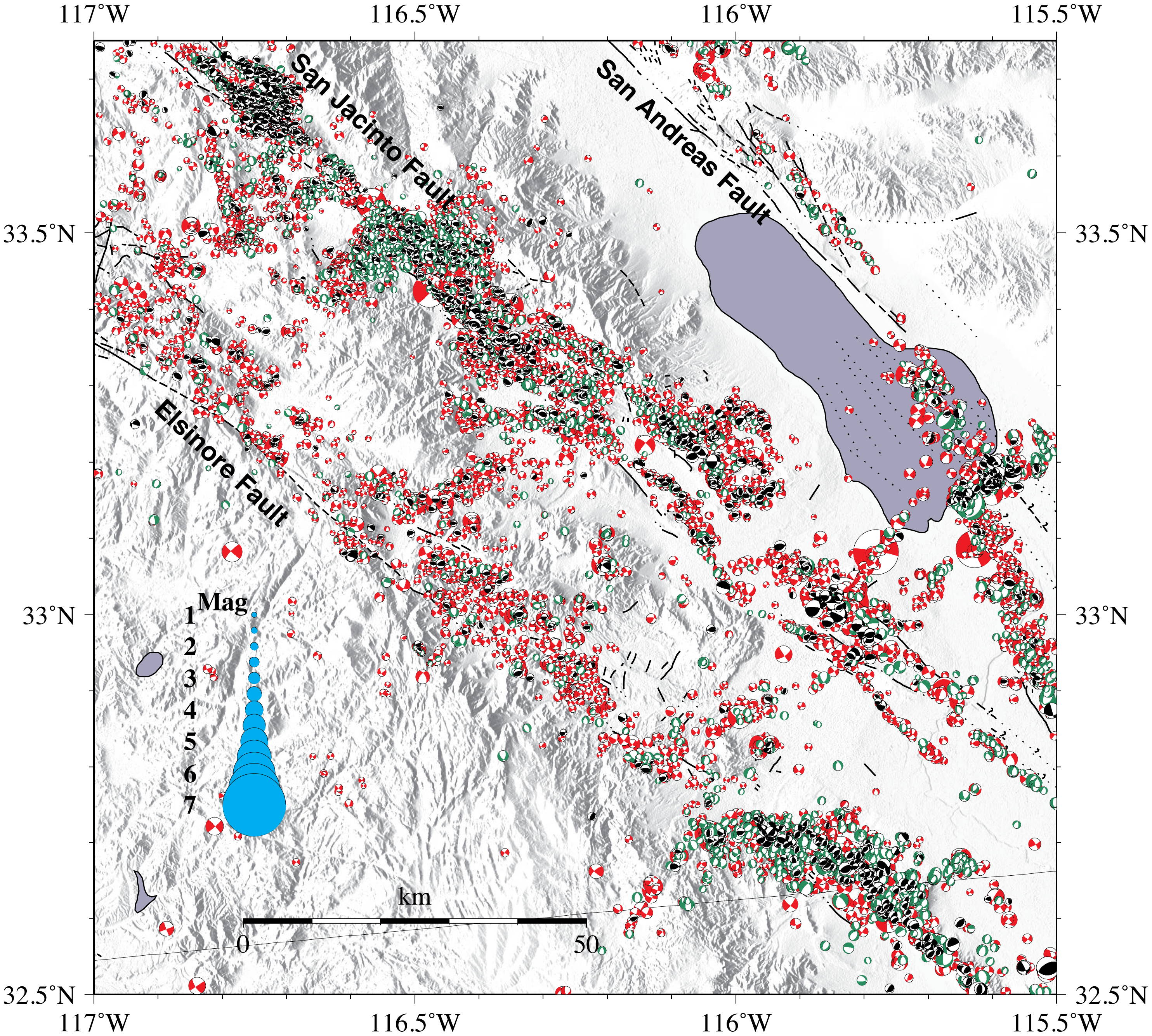
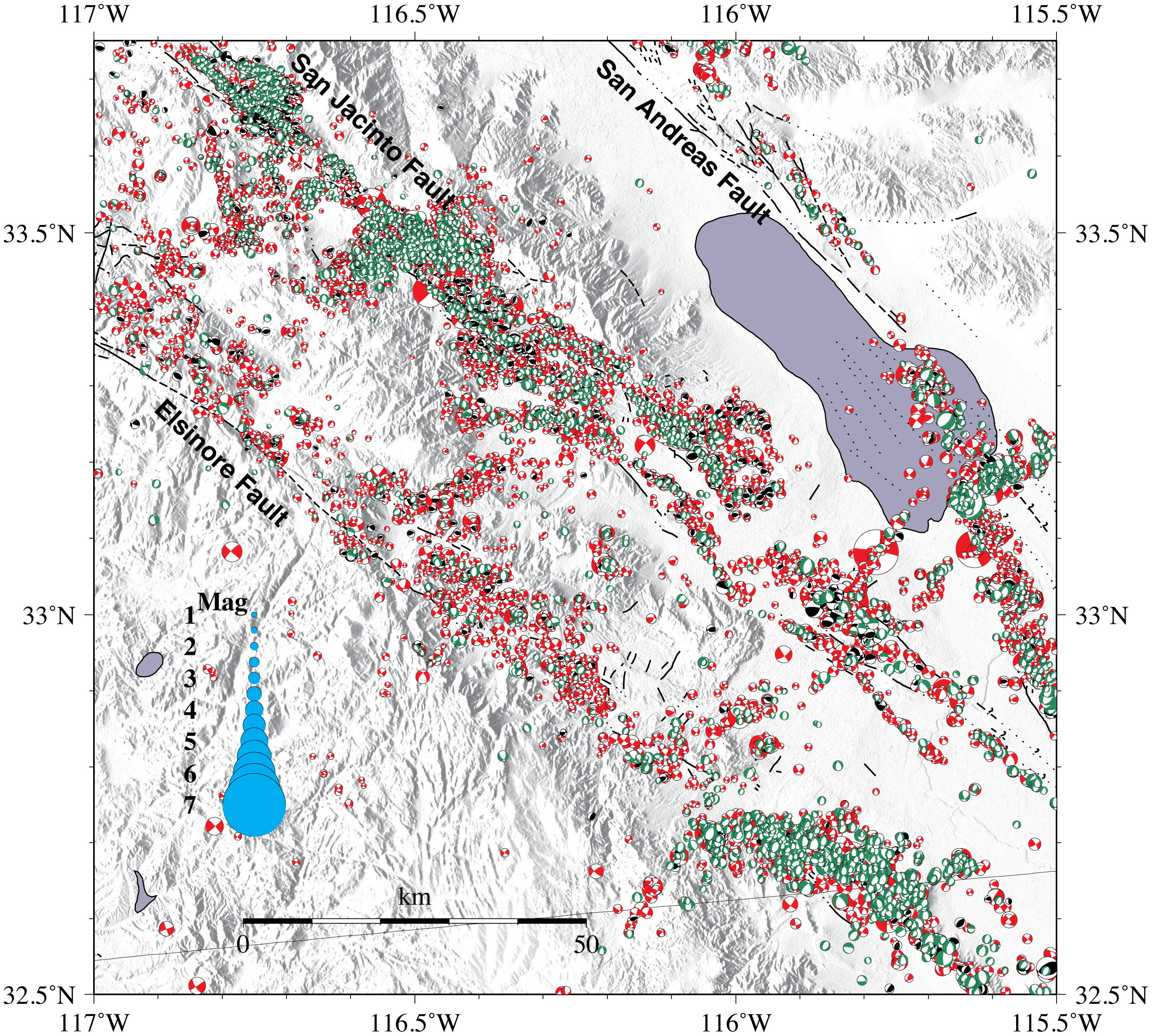
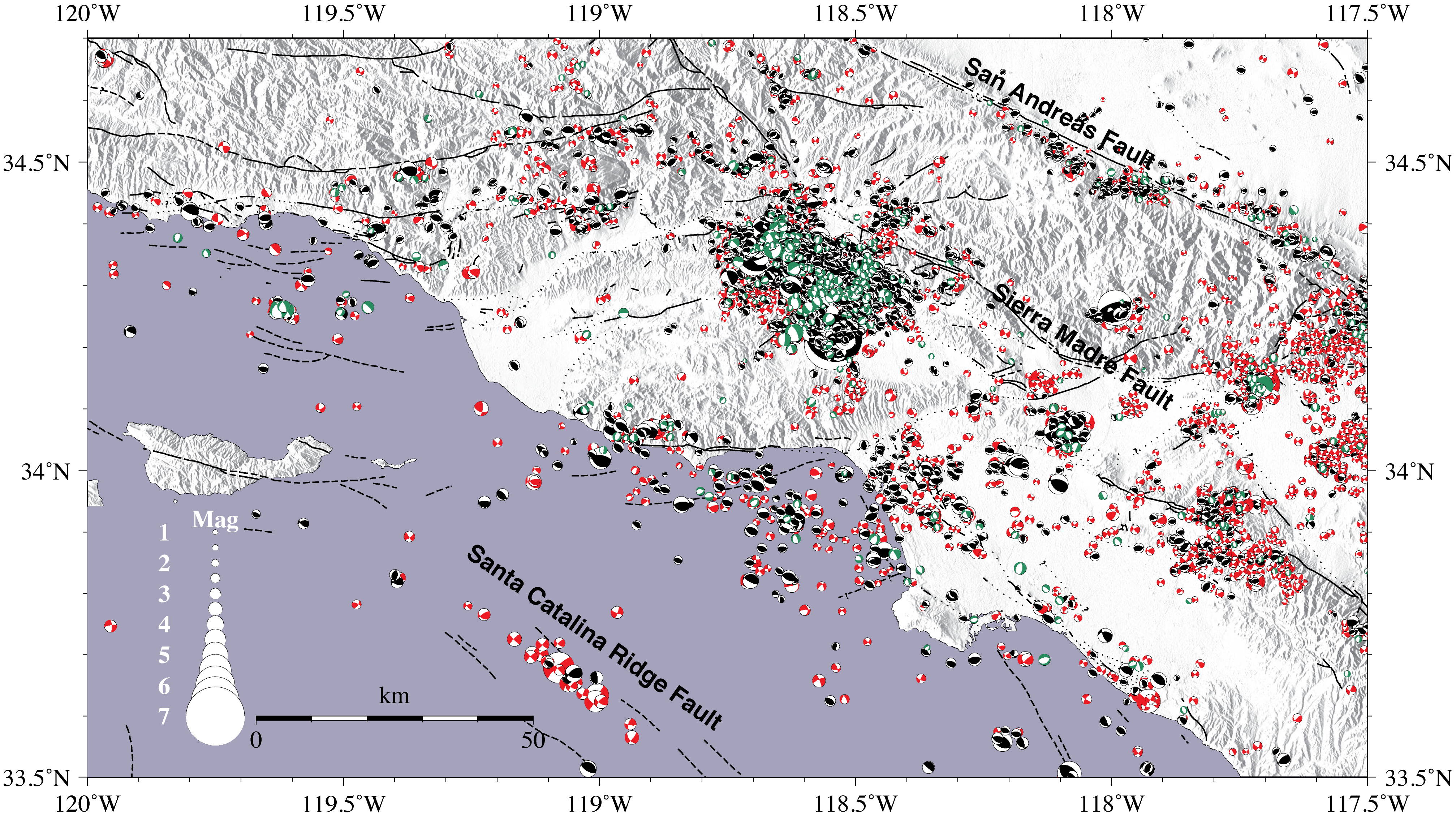
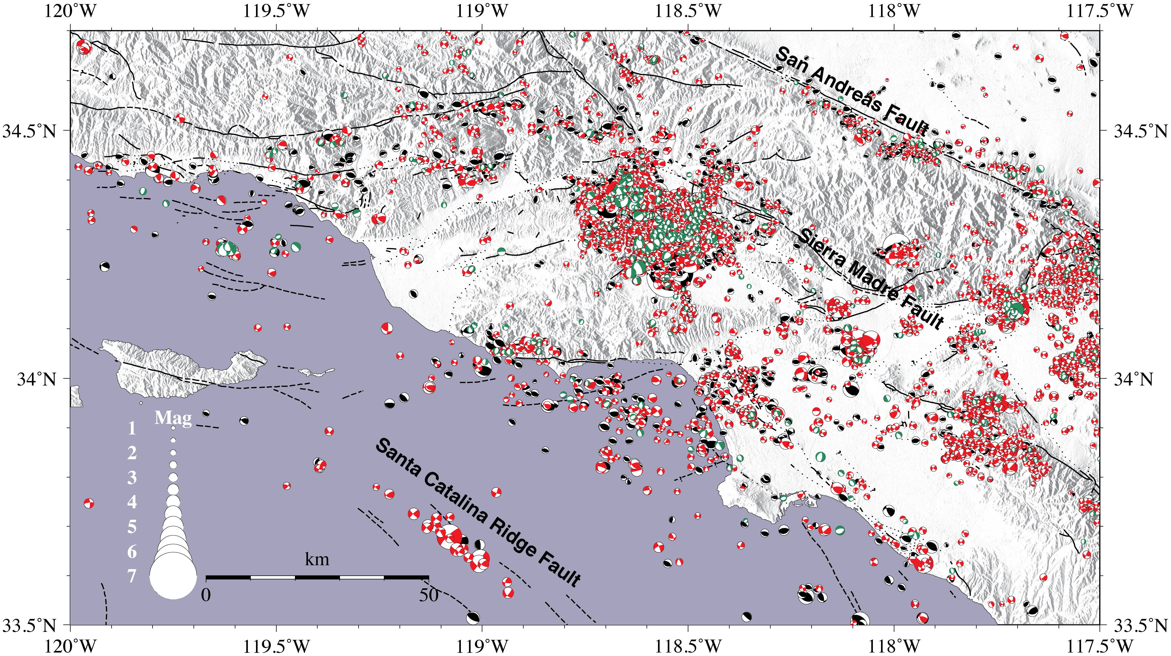
We subdivided the southern California into six regions based on the characteristic tectonic setting and seismicity (Figure S4). For each region, we plotted earthquake focal mechanisms with quality A-C in the YHS2010 focal mechanism catalog (Figure S5-S11). Due to the limitation of map resolution, different styles of faulting could overlap in the same spot. To visualize the data of different faulting styles, we plotted focal mechanisms of different faulting styles with the smallest population of faulting being plotted last. In some areas, there exist nearly equal populations of two styles of faulting; we thereby plotted results in different faulting orders. Thus, we have two separate plots for Region R1 and R2.
Figure S4. The selection of six rectangle regions (R1-R6) in southern California for the visualization of styles of faulting. Faults are plotted as black curves. The insert panel at the top right corner shows the relative location of the map area (red box) in the state of California. The San Andres Fault in bold black curve separates the Pacific Plate and the North America Plate with arrows indicating relative motions.
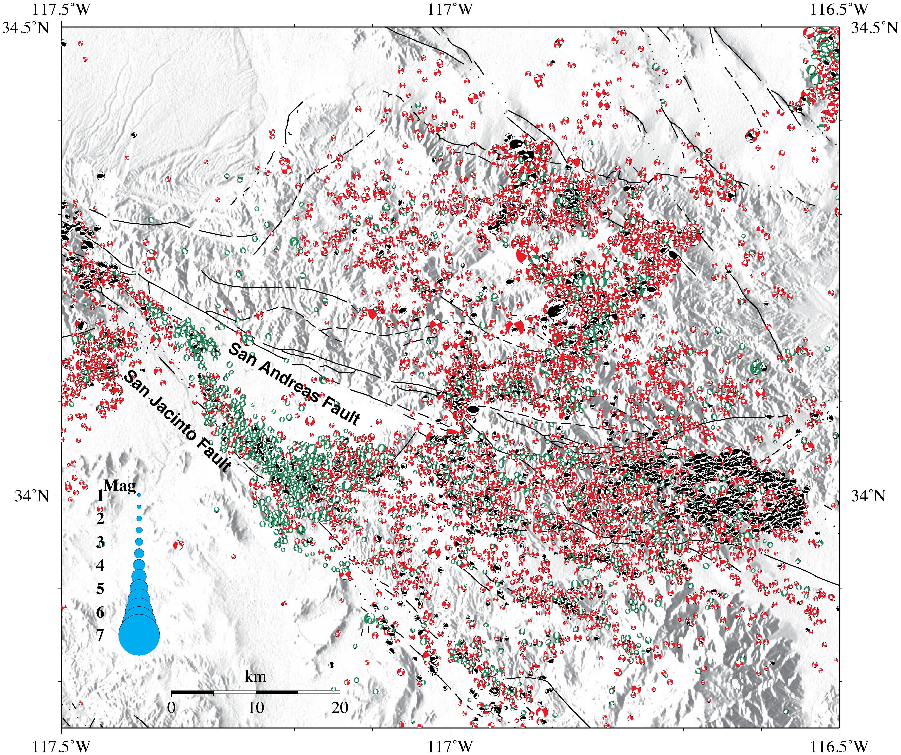
Figure S5a. Map view of quality A-C focal mechanisms in Region R1. Region R1 includes the San Jacinto Fault Zone, the Salton Sea and the Peninsular Ranges. Focal mechanisms are plotted in the order of strike-slip (red), normal (green) and reverse (black). To each style of faulting, events are overlapped temporally. The sizes of beach balls are scaled with magnitudes with legend at the bottom left corner.
Figure S5b. Map view of quality A-C focal mechanisms in Region R1. Focal mechanisms are plotted in the order of strike-slip (red), reverse (black) and normal (green). To each style of faulting, events are overlapped temporally.
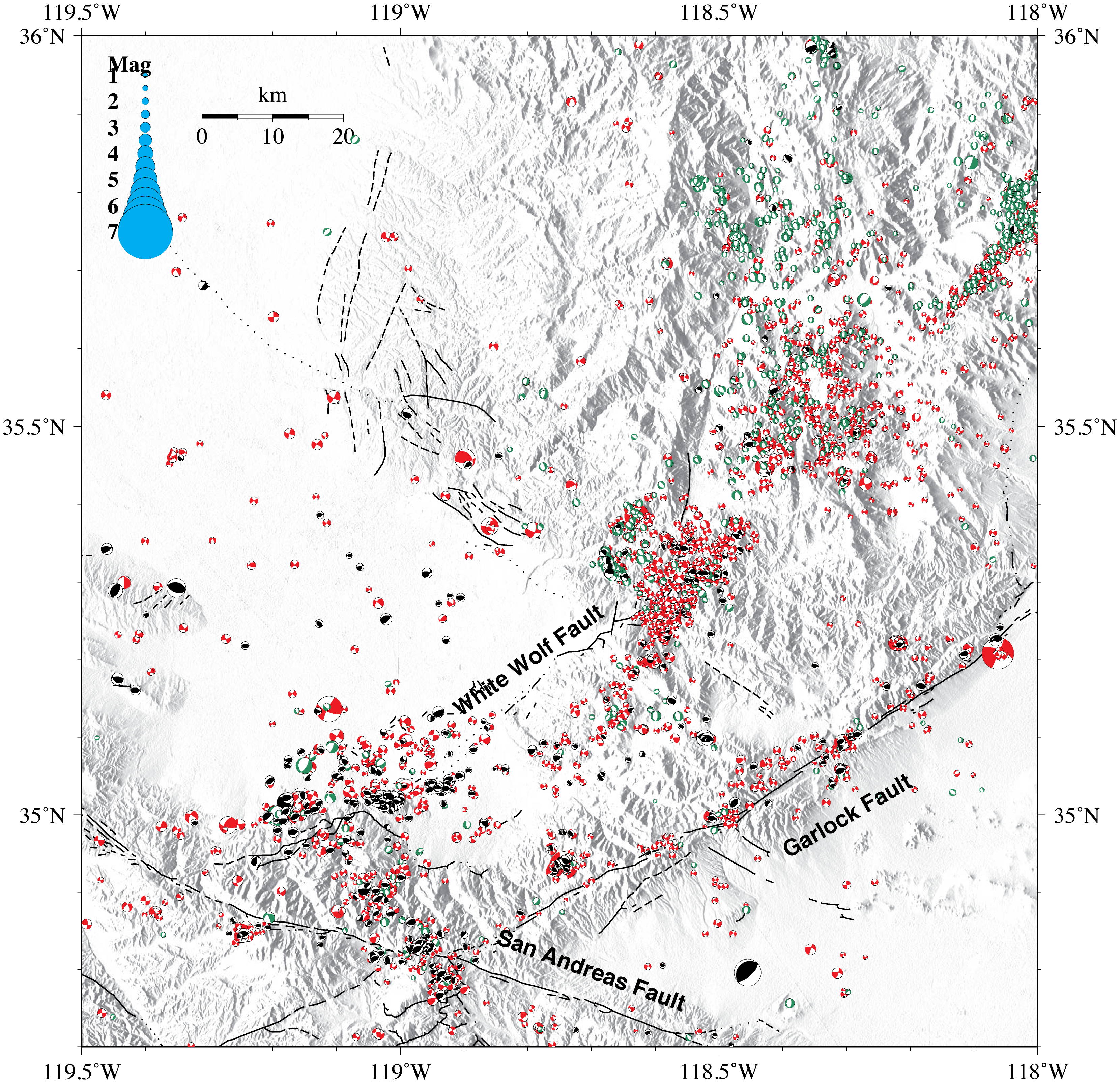
Figure S6a. Map view of quality A-C focal mechanisms in Region R2. Region R2 includes the Transverse Ranges, the San Gabriel Mountains and the LA basin. Focal mechanisms are plotted in the order of strike-slip (red), reverse (black) and normal (green). To each style of faulting, events are overlapped temporally.
Figure S6b. Map view of quality A-C focal mechanisms in Region R2. Focal mechanisms are plotted in the order of reverse (black), strike-slip (red), and normal (green). To each style of faulting, events are overlapped temporally.
Figure S7. Map view of quality A-C focal mechanisms in Region R3. Region R3 includes the San Bernardino Mountains. Focal mechanisms are plotted in the order of strike-slip (red), normal (green) and reverse (black). To each style of faulting, events are overlapped temporally.
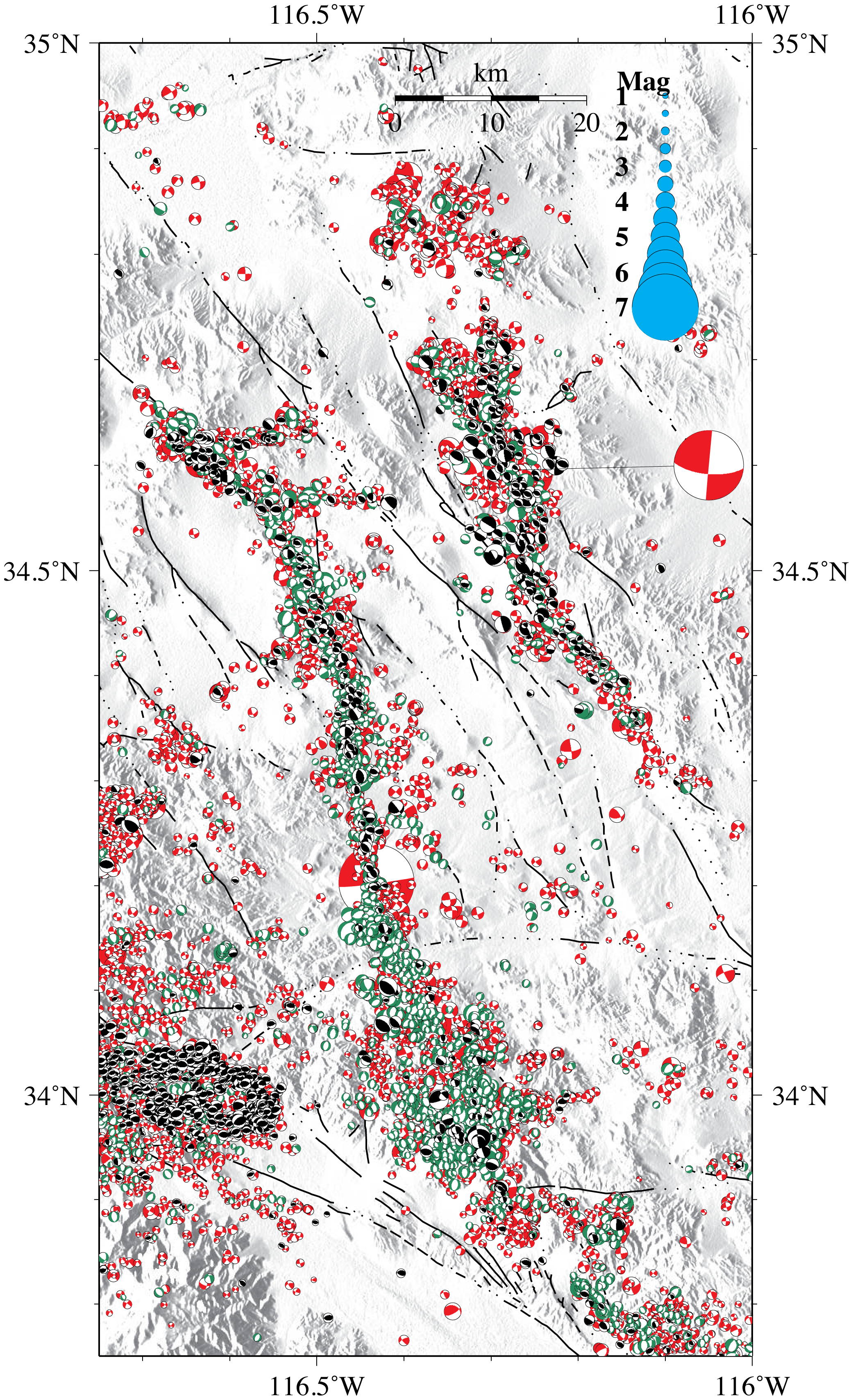
Figure S8. Map view of quality A-C focal mechanisms in Region R4. Region R4 includes the East California Shear Zone. Focal mechanisms are plotted in the order of strike-slip (red), normal (green) and reverse (black). To each style of faulting, events are overlapped temporally. The sizes of beach balls are scaled with magnitudes with legend at the top right corner. The focal mechanism of the 1999 Hector Mine MW7.1 earthquake is marked to the right side.
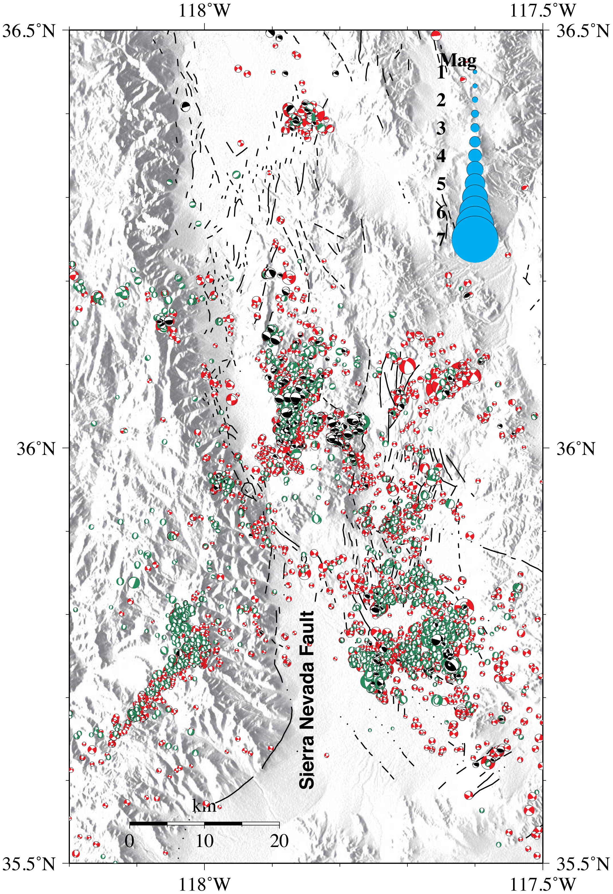
Figure S9. Map view of quality A-C focal mechanisms in Region R5. Region R5 includes the Sierra Nevada. Focal mechanisms are plotted in the order of strike-slip (red), normal (green) and reverse (black). To each style of faulting, events are overlapped temporally. The sizes of beach balls are scaled with magnitudes with legend at the top left corner.
Figure S10. Map view of quality A-C focal mechanisms in Region R6. Region R6 includes the Ridgecrest and the Coso geothermal area. Focal mechanisms are plotted in the order of strike-slip (red), normal (green) and reverse (black). To each style of faulting, events are overlapped temporally. The sizes of beach balls are scaled with magnitudes with legend at the top right corner.
Hauksson, E., (2000). Crustal structure and seismicity distribution adjacent to the Pacific and North America plate boundary in southern California, J. Geophys. Res., 105, 13875-13903.
Shearer, P. M. (1997). Improving local earthquake locations using the L1 norm and waveform cross-correlation: application to the Whittier Narrows, California, aftershock sequence, J. Geophys. Res., 102, 8269-8283.
Hardebeck, J. L., and P. M. Shearer (2003). Using S/P amplitude ratios to constrain the focal mechanisms of small earthquakes, Bull. Seismol. Soc. Am., 93, 2434-2444.
[ Back ]