
Traveltime Tables for iasp91 and ak135
J. Arthur Snoke
Virginia Polytechnic Institute and State University
INTRODUCTION
The purpose of this short paper is to bring attention to the availability of a package for building and applying the traveltime tables as developed by Kennett and Engdahl (1991) for model iasp91 and Kennett et al. (1995) for model ak135. This package has been tested successfully on Linux, Sun Solaris, and Mac OS X. It can be downloaded from the Incorporated Research Institutions for Seismology (IRIS) Data Management Center (DMC) Software—Processing Programs at http://www.iris.edu/software/downloads/processing/.
Kennett and Engdahl (1991) introduced velocity model iasp91, a product of three years of “a major international effort made by the Sub-Commission on Earthquake Algorithms of the International Association of Seismology and the Physics of the Earth’s Interior (IASPEI) to generate new global traveltime tables for seismic phases to update the tables of Jeffreys and Bullen (1940).” The software package to generate and apply these tables was made available to the seismological community by their collaborator, Ray Buland, through a U.S. Geological Survey (USGS) anonymous FTP Web site. Four years later, Kennett, Engdahl, and Buland (1995) produced model ak135, “which gives a significantly better fit to a broad range of phases than is provided by the iasp91 and sp6 models…The differences in velocity between ak135 and these models are generally quite small except at the boundary of the inner core, where reduced velocity gradients are needed to achieve satisfactory performance for PKP differential time data.” In 1996, Buland posted an updated package on the USGS anonymous FTP Web site with the ak135 tables and software to generate and use them. That site has not been accessible for about 10 years.1The text quotes are from the abstracts of the 1991 and 1995 papers. The reference for the sp6 model is Morelli and Dziewonski (1993).
THE iaspei-tau SOFTWARE PACKAGE
In the 1991 Web-accessible software package, the radially stratified velocities and densities were parameterized by polynomial fits within designated layers. In 1991, I decided to use the iasp91-table format for a velocity model that differed from iasp91 in the crust and upper mantle for a study that required the location by a regional network of intermediate-depth (∼150 km) earthquakes (James and Snoke 1994). In developing models, I replaced the polynomial fit with code that read in a velocity-depth model from an ASCII file. This code included options for either linear or cubic-spline interpolation for velocities and densities within layers. Brian Kennett (personal communication) used the linear-interpolation version of this code in the development of model ak135, and a variant of that code is included in Buland’s 1996 Web-accessible version of the software package. Since Kennett used linear interpolation in developing ak135, only that version is used in this package.
As with Buland’s earlier distributions, this distribution of the tables calculates the following family of passes: P, Pdiff, PKP, PKiKP, pP, pPdiff, pPKP, pPKiKP, sP, sPdiff, sPKP, sPKiKP, PP, P’P’, S, Sdiff, SKS, pS, pSdiff, pSKS, sS, sSdiff, sSKS, SS, S’S’, PS, PKS, SP, SKP, SKiKP, PcP, PcS, ScP, ScS, PKKP, PKKS, SKKP, and SKKS.
The package consists of two files: a “tarball” and a README file that has instructions about how to uncompress and expand the tarball file as well as a user’s guide for the package. The package has software for building the tables; an application program, ttimes, that illustrates how to use the tables; Unix-format scripts for the building and testing; and further documentation. The ttimes output files for both the iasp91 and ak135 velocity models include all possible phases from the list given above for the specified focal depths and epicentral distances. Included in the ttimes output is the take-off angle for each phase, a little-advertised feature of the traveltime tables (Ray Buland, personal communication, 2001). The author has found this feature useful in focal-mechanism studies (e.g., Snoke 2003). Output traveltimes are given to 0.001 s, which is more precise than is statistically necessary based on the input velocity-model file entries but facilitates comparisons among models and provides a check of the reproducibility for different compilers and operating systems.
DISCUSSION
The package has been tested successfully on several Unix platforms: Sun Solaris, Linux (both 32-bit and 64-bit native word length), and Mac OS X (both PPC and i686 [Intel]). A Fortran compiler is required. One of the two traveltime-table files is an unformatted sequential-access file, and the convention for such files differs among compilers. It is, therefore, strongly recommended that users build the tables using the same Fortran compiler, on the same platform, on which the analysis programs (such as ttimes) are compiled.2The version of the compiler can make a difference; the convention for unformatted sequential access file records was changed in version 4.2 of the gfortran compiler.
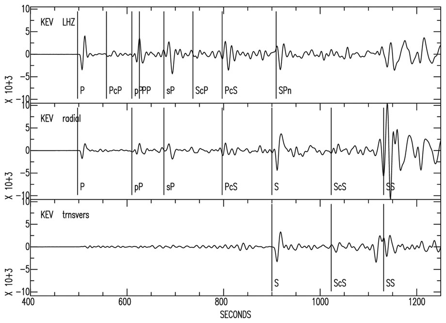
▲ Figure 1. The waveforms were downloaded from the IRIS DMC database and are unprocessed LH components sampled at 1 sps. The radial and transverse components are calculated from LHN and LHE. Arrival times are calculated by program ttimes for model iasp91 assuming a focal depth of 611 km and an epicentral distance of 52.474°. As noted in the text, the phase sPP is predicted to arrive about three seconds before PcS; based on the observed particle motion, sPP is a better fit for the observed arrival. Click image to view a larger version.
Hellfrich (2008) independently developed the iaspei-tau routines, principally to supply them with a computational subroutine interface. (The routines underlie the slant stacking and receiver function processing methods.) Additional modifications include providing tables for Earth models in addition to ak135 and iasp91 (PREM at 1 s and 20 s, sp6, kghj, pemc), additional depth phase arrival times, and inner-core diffractions. The traveltime table format produced by Hellfrich’s package is not compatible with the iaspei-tau layouts published by the original authors and included in this iaspei-tau package. The changed format makes the table sizes self-describing and eliminates their dependence on dimensions set at model-building time. Hellfrich’s package contains source code and an automatic configure script for quick installation; customizing the installation is also possible (Hellfrich, personal communication, 2008).
An alternative to the iasp91-format traveltime tables is Crotwell’s TauP Toolkit (Crotwell et al. 1999). As with Kennett and Engdahl (1991), the method used is based on the calculating scheme proposed by Buland and Chapman (1983). The TauP Toolkit is written in Java. It includes several models in addition to iasp91 and ak135. The following command line produces output that can be compared with one of the ttimes runs in this package:
taup_time -model ak135 -h 300 -deg 150 -ph ttall
A common application of traveltime tables is predicting and plotting arrival times for body-wave phases at one or more stations from earthquakes. Usually this is done automatically, using a program like ttimes in collaboration with a package like SAC (Goldstein et al. 2003). Figure 1 shows an example: seismograms from station KEV: 52.474° from the epicenter of the deep-focus (611 km) 12 May 1990 Sakhalin Island event. This set of seismograms was chosen because of the large number of clear body-wave arrivals. In preparing Figure 1, the arrival times were calculated using program ttimes for model iasp91 and (manually) included using a SAC script. A close examination of the arrival labeled PcS shows that care must be taken when interpreting predicted arrival times: A phase that arrives as an S should be out of phase on the vertical and radial components, and, based on the predicted emergence angle of 7.6°, the amplitude on the radial should be 6.5 times as large as the amplitude on the vertical. Yet as seen in Figure 1, the arrivals are clearly in phase on the vertical and radial, and the amplitude ratio is 0.4. Hence the arrival must be a P phase at KEV. George Hellfrich (personal communication 2008) suggested that the arrival might be sPP, and he noted that several “depth phases” of interest to him are not included among the calculated phases for this distribution. A run with taup_time for this geometry using the iasp91 model supports Hellfrich’s suggestion: sPP is predicted to arrive about three seconds before the predicted arrival time for PcS. (The phase sPP, however, is not included in Hellfrich’s (2008) package). ![]()
ACKNOWLEDGMENTS
The author thanks R. Buland, R. Engdahl, B. Kennett, and G. Hellfrich for conversations and e-mail exchanges over the years about traveltime tables. He also thanks IRIS for hosting this package.
REFERENCES
Buland, R., and C. H. Chapman (1983). The computation of seismic travel times. Bulletin of the Seismological Society of America 73, 1,271–1,302.
Crotwell, H. P., T. J. Owens, and J. Ritsema (1999). The TauP Toolkit: Flexible seismic travel-time and ray-path utilities. Seismological Research Letters 70, 154–160. The package can be downloaded from http://www.seis.sc.edu/TauP/.
Goldstein, P., D. Dodge, M. Firpo, and L. Minner (2003). SAC2000: Signal processing and analysis tools for seismologists and engineers. International Handbook of Earthquake and Engineering Seismology, ed. W. H. K. Lee, H. Kanamori, P. C. Jennings, and C. Kisslinger, chapter 85.5 San Diego: Academic Press. Those in the IRIS community can download the software package at http://www.iris.edu/software/sac/.
Hellfrich, G. (2008). Buland and Kennett Tau-P travel time calculation routines. Available through http://www1.gly.bris.ac.uk/~george/sac-bugs.html.
James, D. E., and J. A. Snoke (1994). Structure and tectonics in the region of flat subduction beneath central Peru. Part I: Crust and uppermost mantle. Journal of Geophysical Research 99, 6,899–6,912.
Jeffreys, H., and K.E. Bullen (1940). Seismological Tables. London: British Association for the Advancement of Science.
Kennett, B. L. N., and E. R. Engdahl (1991). Traveltimes for global earthquake location and phase identification. Geophysical Journal International 122, 429–465.
Kennett, B. L. N., E. R. Engdahl, and R. Buland (1995). Constraints on seismic velocities in the Earth from traveltimes. Geophysical Journal International 122, 108–124.
Morelli, A., and A. M. Dziewonski (1993). Body-wave traveltimes and a spherically symmetric P- and S-wave velocity model. Geophysical Journal International 112, 178–184.
Snoke, J. A. (2003). FOCMEC: FOcal MEChanism determinations. International Handbook of Earthquake and Engineering Seismology, ed. W. H. K. Lee, H. Kanamori, P. C. Jennings, and C. Kisslinger, chapter 85.12. San Diego: Academic Press. The software package can be downloaded from the IRIS DMC Software—Processing Programs at http://www.iris.edu/software/downloads/processing/.
Footnotes
1 The text quotes are from the abstracts of the 1991 and 1995 papers. The reference for the sp6 model is Morelli and Dziewonski (1993).
2 The version of the compiler can make a difference; the convention for unformatted sequential access file records was changed in version 4.2 of the gfortran compiler.
[ Back ]
Posted: 13 March 2009