
ObsPy: A Python Toolbox for Seismology
Moritz Beyreuther,1 Robert Barsch,1 Lion Krischer,1 Tobias Megies,1 Yannik Behr,2 and Joachim Wassermann1
 Authors' Affiliations") Click to Show (or Hide) Authors' Affiliations
Click to Show (or Hide) Authors' Affiliations
- Department of Earth and Environmental Sciences, Geophysical Observatory, Ludwig Maximilians Universität München, Germany
- School of Geography, Environment, and Earth Sciences, Victoria University of Wellington, New Zealand
INTRODUCTION
The wide variety of computer platforms, file formats, and methods to access seismological data often requires considerable effort in preprocessing such data. Although preprocessing work-flows are mostly very similar, few software standards exist to accomplish this task. The objective of ObsPy is to provide a Python toolbox that simplifies the usage of Python programming for seismologists. It is conceptually similar to SEATREE (Milner and Thorsten 2009) or the exploration seismic software project MADAGASCAR (http://www.reproducibility.org). In ObsPy the following essential seismological processing routines are implemented and ready to use: reading and writing data only SEED/MiniSEED and Dataless SEED (http://www.iris.edu/manuals/SEEDManual_V2.4.pdf), XML-SEED (Tsuboi et al. 2004), GSE2 (http://www.seismo.ethz.ch/autodrm/downloads/provisional_GSE2.1.pdf) and SAC (http://www.iris.edu/manuals/sac/manual.html), as well as filtering, instrument simulation, triggering, and plotting. There is also support to retrieve data from ArcLink (a distributed data request protocol for accessing archived waveform data, see Hanka and Kind 1994) or a SeisHub database (Barsch 2009). Just recently, modules were added to read SEISAN data files (Havskov and Ottemöller 1999) and to retrieve data with the IRIS/FISSURES data handling interface (DHI) protocol (Malone 1997).
Python gives the user all the features of a full-fledged programming language including a large collection of scientific open-source modules. ObsPy extends Python by providing direct access to the actual time series, allowing the use of powerful numerical array-programming modules like NumPy (http://numpy.scipy.org) or SciPy (http://scipy.org). Results can be visualized using modules such as matplotlib (2D) (Hunter 2007) or MayaVi (3D) (http://code.enthought.com/projects/mayavi/). This is an advantage over the most commonly used seismological analysis packages SAC, SEISAN, SeismicHandler (Stammler 1993), or PITSA (Scherbaum and Johnson 1992), which do not provide methods for general numerical array manipulation.
Because Python and its previously mentioned modules are open-source, there are no restrictions due to licensing. This is a clear advantage over the proprietary product MATLAB (http://www.mathworks.com) in combination with MatSeis (Creager 1997) or CORAL (Harris and Young 1997), where the number of concurrent processes is limited by a costly and restricting license policy. Additionally, Python is known for its intuitive syntax. It is platform independent, and its rapidly growing popularity extends beyond the seismological community (see, e.g., Olsen and Ely 2009). Python is used in various fields because its comprehensive standard library provides tools for all kinds of tasks (e.g., complete Web servers can be written in a few lines with standard modules). It has excellent features for wrapping external shared C or FORTRAN libraries, which are used within ObsPy to access libraries for manipulating MiniSEED (libmseed; http://www.iris.edu/pub/programs) and GSE2 (gse_util; http://www.orfeus-eu.org/Software/softwarelib.html#gse) volumes. Similarly, seismologists may wrap their own C or FORTRAN code and thus are able to quickly develop powerful and efficient software.
In the next section we will briefly introduce the capabilities of ObsPy by demonstrating the data conversion of SAC files to MiniSEED volumes, removing the instrument response, applying a low-pass filter, and plotting the resulting trace. We then give an overview on how to access an external C or FORTRAN library from within Python.
from obspy.core import UTCDateTime
from obspy.arclink import Client
from obspy.signal import cornFreq2Paz, seisSim, lowpass
import numpy as np, matplotlib.pyplot as plt
#1 Retrieve Data via Arclink
client = Client(host=”webdc.eu”, port=18001)
t = UTCDateTime(“2009-08-24 00:20:03”)
one_hertz = cornFreq2Paz(1.0) # 1Hz instrument
st = client.getWaveform(“BW”, “RJOB”, “”, “EHZ”, t, t+30)
paz = client.getPAZ(“BW”, “RJOB”, “”, “EHZ”, t, t+30).values()[0]
#2 Correct for frequency response of the instrument
res = seisSim(st[0].data.astype(“float32”), st[0].stats.sampling_rate, paz, inst_sim=one_hertz)
# Correct for overall sensitivity, nm/s
res *= 1e9 / paz[“sensitivity”]
#3 Apply lowpass at 10Hz
res = lowpass(res, 10, df=st[0].stats.sampling_rate, corners=4)
#4 Plot the seismograms
sec = np.arange(len(res))/st[0].stats.sampling_rate
plt.subplot(211)
plt.plot(sec,st[0].data, “k”)
plt.title(“%s %s” % (“RJOB”,t))
plt.ylabel(“STS-2”)
plt.subplot(212)
plt.plot(sec,res, “k”)
plt.xlabel(“Time [s]”)
plt.ylabel(“1Hz CornerFrequency”)
plt.show()
▲ Figure 1. Advanced example. Data as well as the instrument response are fetched via ArcLink (please note the ArcLink server at http://webdc.eu is sometimes unreachable). A seismometer with 1 Hz corner frequency is simulated and the resulting data are lowpassed at 10 Hz. An example of the original and the resulting data is plotted and shown in Figure 2.
READING AND WRITING
ObsPy provides unified access to read seismograms formatted as GSE2, MiniSEED, SAC, or SEISAN. For example, entering the following code in a Python shell/interpreter
>>> from obspy.core import read
>>> st = read("my_file")
automatically detects the file format and loads the data into a stream object that consists of multiple trace objects itself. In MiniSEED as well as in GSE2, multiple data records can be stored into one single file. These separate data records are each read into one trace object.
The header attributes of the first trace (tr = st[0]) can be addressed by the tr.stats object (e.g., tr.stats.sampling_rate). The attribute tr.data contains the data as a numpy.ndarray object (array-programming). Thus the data can be further processed by standard Python, NumPy, SciPy, matplotlib, or ObsPy routines, e.g., by applying NumPy’s fast Fourier transform for real valued data:
>>> import numpy
>>> print numpy.fft.rfft(tr.data - tr.data.mean())
For a conversion from one file format to another, the write method of the stream object can be used:
>>> from obspy.core import read
>>> st = read("my_file.sac")
>>> st.write(“my_file.mseed”,format=“MSEED”)
By using the concept of streams and traces, we will introduce more functions of ObsPy through the following undergraduate homework example.
AN UNDERGRADUATE-LEVEL EXERCISE
The task is to extract 30 s data via ArcLink from WebDC (http://webdc.eu) (Figure 1, #1), deconvolve the instrument response, and simulate an instrument with 1 Hz corner frequency (Figure 1, #2). The corrected trace should be low-passed at 10 Hz (Figure 1, #3) and plotted together with the original seismogram (Figure 1, #4 and Figure 2).
The example in Figure 1 can be extended by fetching data from two different stations, preprocessing them in the same way as in Figure 1, and then directly passing the resulting traces to a custom cross-correlation function written in C. We will provide the technical details on how to wrap the custom crosscorrelation function or any other C or FORTRAN function in the next section.
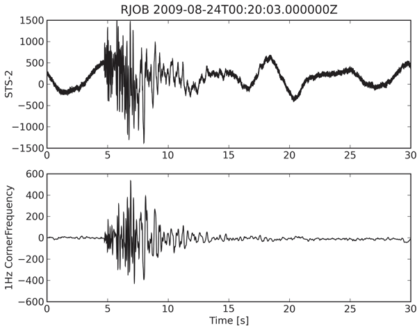
▲ Figure 2. Local earthquake recorded at station RJOB. The top figure shows the STS-2 instrument. The bottom figure shows the simulated instrument with 1Hz corner frequency low-pass filtered at 10 Hz.
Extending Python with a Custom Shared Library
In general, interpreters (e.g., Python, Perl, R, MATLAB) are considered slower than compiled source code (e.g., C, FORTRAN). Therefore performance can be optimized by transferring routines with time critical code from Python to compiled shared libraries. Python’s foreign function library “ctypes” enabled the ObsPy developers to pass data from Python to functions in shared C or FORTRAN libraries. In doing so the Python memory is accessed directly from the C or FORTRAN function, so that no memory copying is necessary. Furthermore, the complete interface part is written in the interpreter language (no modification of the C code) which makes it easy to reuse existing code.
An example of how to access the custom cross-correlation C function
void X_corr(float *tr1, float *tr2, int param, int ndat1, \
int ndat2, int *shift, double* coe_p)
from Python is provided in Figure 3 (please note that a standard cross-correlation is also included in SciPy).
In lines 1 and 2 of the program (Figure 3) the modules and the shared library are loaded (.so typically stands for a shared library on Linux; this may vary for other operating systems). In lines 4 and 5, pointers to hold the resulting shift and cross-correlation coefficient are allocated and passed to the C function in lines 6 and 7. Note that data1 and data2 need to be numpy. ndarrays of type “float32” (type checking is included in ctypes but omitted in the example for simplicity). The values of the pointers can now be accessed via the attributes shift.value and coe_p.value.
At this point we want to emphasize that this interface design differs from MATLAB, where the interfaces need to be written in the compiled language (MEX-files).
1 import ctypes as C
2 lib = C.CDLL(“pathto”+”xcorr.so”)
3 #
4 shift = C.c_int()
5 coe_p = C.c_double()
6 lib.X_corr(data1.ctypes.data_as(C.POINTER(C.c_float)), data2.ctypes.data_as(C.POINTER(C.c_float)),
7            window_len, len(data1), len(data2), C.byref(shift), C.byref(coe_p))
▲ Figure 3. C interface for accessing the shared library xcorr.so from the Python side using ctypes. The resulting shift and correlation coefficient can be accessed via the attributes shift.value and coe_p.value.
DISCUSSION AND CONCLUSION
The intent behind ObsPy is not to provide complete seismological analysis software but to give seismologists access to the basic functionalities they need to use Python to easily combine their own programs (Python libraries, modules written in C/ FORTRAN). It could also be seen as a nucleation point for a standard seismology package in Python. Key factors justifying continuation of the ObsPy package are: test-driven development (currently containing 304 tests), modular structure, reliance on well-known third-party tools where possible, opensource code, and platform independency (Win, Mac, Linux). The ObsPy package and detailed documentation can be accessed at http://www.obspy.org. We encourage any interested user to develop new functions and applications and to make them available via the central repository — https://svn.geophysik.uni-muenchen.de/svn/obspy/. We believe that such a free and open-source development environment, backed up by Python, makes ObsPy a useful toolbox for many seismologists.
ACKNOWLEDGMENTS
We want to thank Heiner Igel and Christian Sippl for their kind support. We also thank Chad Trabant, Stefan Stange, and Charles J. Ammon, whose libraries are the basis for the MiniSEED, GSE2, and SAC support, respectively. The suggestions of Kim Olsen substantially improved the manuscript. This work was partially funded by the German Ministry for Education and Research (BMBF), GEOTECHNOLOGIEN grant 03G0646H.
REFERENCES
Barsch, R. (2009). Web-based technology for storage and processing of multi-component data in seismology. PhD thesis, Ludwig Maximilians Universität München, Munich, Germany.
Creager, K. (1997). CORAL. Seismological Research Letters 68 (2), 269–271.
Hanka, W., and R. Kind (1994). The GEOFON program. Annali di Geofisica 37 (5), 1,060–1,065.
Harris, M., and C. Young (1997). MatSeis: A seismic GUI and toolbox for Matlab. Seismological Research Letters 68 (2), 267–269.
Havskov, J., and L. Ottemöller (1999). SEISAN earthquake analysis software. Seismological Research Letters 70 (5), 522–528.
Hunter, J. D. (2007). Matplotlib: A 2D graphics environment. Computing in Science and Engineering 3 (9), 90–95.
Malone, S. (1997). Electronic seismologist goes to FISSURES. Seismological Research Letters 68 (4), 489–492
Milner, K., and W. Thorsten (2009). New software framework to share research tools. Eos, Transactions, American Geophysical Union 90 (12), 104; http://geosys.usc.edu/projects/seatree.
Olsen, K. B., and G. Ely (2009). WebSims: A web-based system for storage, visualization, and dissemination of earthquake ground motion simulations. Seismological Research Letters 80, 1,002–1,007.
Scherbaum, F., and J. Johnson (1993). PITSA, Programmable Interactive Toolbox for Seismological Analysis. Technical report, IASPEI Software Library.
Stammler, K. (1993). SeismicHandler—programmable multichannel data handler for interactive and automatic processing of seismological analyses. Computers & Geosciences 19 (2), 135–140.
Tsuboi, S., J. Tromp, and D. Komatitsch (2004). An XML-SEED format for the exchange of synthetic seismograms. Eos, Transactions, American Geophysical Union SF31B-03.
[ Back ]
Posted: 04 May 2010 · Updated: 20 May 2010