
The SCEC/USGS Dynamic Earthquake Rupture Code Verification Exercise
R. A. Harris,1* M. Barall,1,2 R. Archuleta,3 E. Dunham,4 B. Aagaard,1 J. P. Ampuero,5 H. Bhat,6 V. Cruz-Atienza,7 L. Dalguer,8 P. Dawson,1 S. Day,9 B. Duan,1 G. Ely,6 Y. Kaneko,5 Y. Kase,11 N. Lapusta,5 Y. Liu,5 S. Ma,9 D. Oglesby,12 K. Olsen,9 A. Pitarka,13 S. Song,13 and E. Templeton4
 Authors' Affiliations") Click to Show (or Hide) Authors' Affiliations
Click to Show (or Hide) Authors' Affiliations
- U.S. Geological Survey, Menlo Park, California, U.S.A.
- Invisible Software, San Jose, California, U.S.A.
- University of California, Santa Barbara, U.S.A.
- Harvard University, Cambridge, Massachusetts, U.S.A.
- California Institute of Technology, Pasadena, California, U.S.A.
- University of Southern California, Los Angeles, U.S.A.
- Universidad Nacional Autónoma de México, Mexico City, Mexico
- ETH, Zurich, Switzerland
- San Diego State University, California, U.S.A.
- Texas A & M University, College Station, Texas, U.S.A.
- Geological Survey of Japan, Tsukuba, Japan
- University of California, Riverside, U.S.A.
- URS Corporation, Pasadena, California, U.S.A.
INTRODUCTION
Numerical simulations of earthquake rupture dynamics are now common, yet it has been difficult to test the validity of these simulations because there have been few field observations and no analytic solutions with which to compare the results. This paper describes the Southern California Earthquake Center/ U.S. Geological Survey (SCEC/USGS) Dynamic Earthquake Rupture Code Verification Exercise, where codes that simulate spontaneous rupture dynamics in three dimensions are evaluated and the results produced by these codes are compared using Web-based tools. This is the first time that a broad and rigorous examination of numerous spontaneous rupture codes has been performed—a significant advance in this science. The automated process developed to attain this achievement provides for a future where testing of codes is easily accomplished.
Scientists who use computer simulations to understand earthquakes utilize a range of techniques. Most of these assume that earthquakes are caused by slip at depth on faults in the Earth, but hereafter the strategies vary. Among the methods used in earthquake mechanics studies are kinematic approaches and dynamic approaches.
The kinematic approach uses a computer code that prescribes the spatial and temporal evolution of slip on the causative fault (or faults). These types of simulations are very helpful, especially since they can be used in seismic data inversions to relate the ground motions recorded in the field to slip on the fault(s) at depth. However, these kinematic solutions generally provide no insight into the physics driving the fault slip or information about why the involved fault(s) slipped that much (or that little). In other words, these kinematic solutions may lack information about the physical dynamics of earthquake rupture that will be most helpful in forecasting future events.
To help address this issue, some researchers use computer codes to numerically simulate earthquakes and construct dynamic, spontaneous rupture (hereafter called “spontaneous rupture”) solutions. For these types of numerical simulations, rather than prescribing the slip function at each location on the fault(s), just the friction constitutive properties and initial stress conditions are prescribed. The subsequent stresses and fault slip spontaneously evolve over time as part of the elasto-dynamic solution. Therefore, spontaneous rupture computer simulations of earthquakes allow us to include everything that we know, or think that we know, about earthquake dynamics and to test these ideas against earthquake observations.
INGREDIENTS OF A SPONTANEOUS RUPTURE EARTHQUAKE SIMULATION
There are a number of ingredients (assumptions) in a spontaneous rupture earthquake simulation (e.g., see Harris 2004 for an overview; Figure 1). These include the geometry of the fault(s) involved, the properties of the materials that surround and comprise the fault zone, the initial stress conditions, and the failure criterion (fault constitutive relation) that specifies the coseismic friction and determines whether or not points on the fault will be allowed to slip. Whereas the geometry and the on-fault and off-fault material properties may be inferred using detailed field investigations of the Earth’s crust, the initial stress conditions and fault constitutive relation remain, to this date, elusive aspects of coseismic earthquake-faulting behavior. There are, however, numerous ideas for both coseismic friction and stress conditions presented in the literature that are based on laboratory experiments and inferences from field observations, respectively (for an overview on coseismic friction hypotheses, see Tullis 2007).
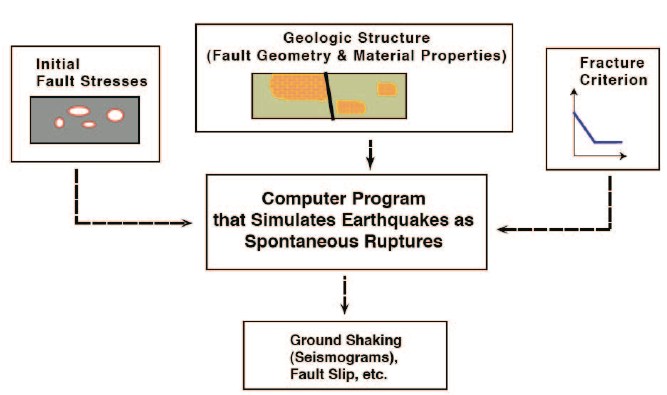
▲ Figure 1. Ingredients of a spontaneous rupture simulation include the initial shear and normal stresses, the on-fault and off-fault material properties, the fault geometry, and the failure criterion that allows the fault to slip. Once all of these are assigned, a computer code that simulates spontaneous rupture is used to calculate results such as the earthquake rupture’s progress, the time-dependent fault slip, the resulting earthquake magnitude, and synthetic seismograms throughout the medium. Figure slightly modified from Harris and Archuleta (2004).
HOW TO TEST A SPONTANEOUS RUPTURE COMPUTER SIMULATION
The most challenging aspect of spontaneous rupture computer simulations of earthquakes is that even if one does know the exact forms of the fault geometry, the material properties, the initial stresses, and the friction, the computer codes themselves still cannot be rigorously tested against analytic solutions (closed form equations for the resulting motions), because no analytic solutions exist for any realistic earthquake scenario. So although newly developed spontaneous rupture codes are often tested against one or two existing analytic solutions, these analytic solutions are only for very simple, unrealistic scenarios. An example is the analytic solution for an earthquake that starts slipping a fault at a constant speed and continues to rupture the fault forever at that speed (Kostrov 1964; also see Madariaga 2007 for a full explanation of this approach). Once these unrealistic, but mathematically possible, scenarios are tested, the code user (“modeler”) starts to have confidence that his/her code behaves in a promising manner; nevertheless, this is not enough.
Until now, most modelers’ next steps have been to either compare the results of their spontaneous rupture codes with intuition, which can be risky since we really don’t understand earthquakes that well, or to compare the results of their codes with those of other codes (preferably by other authors) simulating the same earthquake rupture scenario. Three decades ago, when there were few people working in this area of spontaneous rupture dynamics and there was a scarcity of computational resources, the comparison exercise was challenging at best. Sometimes it was not clear which solution was correct, and rarely, if ever, were careful comparisons made between different authors’ codes using the same assumptions about fault and rupture mechanics. Nowadays however, there are both abundant computational resources and abundant computer codes, so comparison is both desirable and possible (e.g., Day et al., 2005; Moczo et al., 2007). The goal of the SCEC/USGS Rupture Dynamics Code Validation group is to compare the computer codes used by SCEC and USGS researchers to simulate earthquake source physics, and to verify that these codes are functioning as expected.
We are currently testing and comparing 16 spontaneous rupture computer codes developed by more than 18 authors in the SCEC/USGS code validation exercises. We only consider codes that model the Earth in three dimensions. Although it is much more computationally efficient and often more mathematically elegant to consider two-dimensional rupture simulations, we have restricted our comparisons to the 3D codes. These 3D codes have many advantages, including their ability to simulate synthetic seismograms (and synthetic geodetic and geologic slip measurements) at the Earth’s surface that can then be compared with observed seismograms, GPS station movement, and geologic field offsets. 3D simulations also allow us to include the 3D heterogeneity in fault geometry and fault rheology that we know exist in the real Earth.
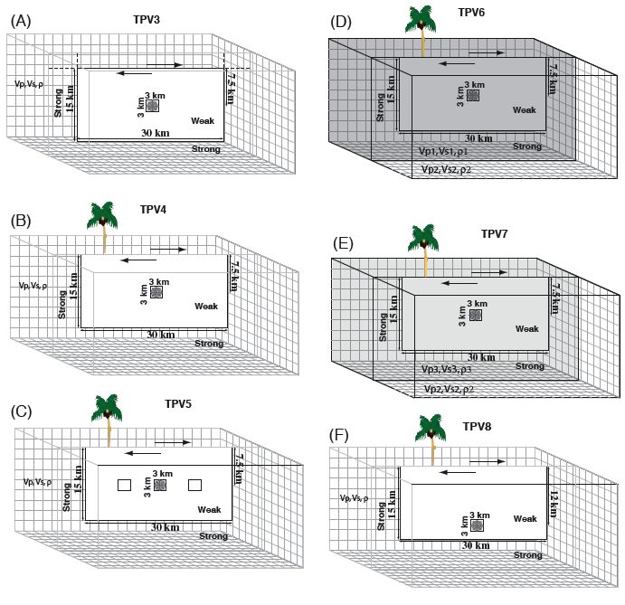
▲ Figure 2. The progression of benchmarks in our code verification exercise. (A) Our first rigorously defined benchmark has slip-weakening friction and rupture on a stress-homogeneous vertical strike-slip fault set in a homogeneous (material properties) full-space (TPV3) The initial shear and normal stresses are assigned to be homogeneous for the 30-km-long by 15-km-deep fault, with the exception of the nucleation zone that has higher initial shear stresses. To stop the rupture from continuing far beyond the 30-km by 15-km fault boundaries, the yield strength is set to a high value, so that the fault is strong beyond these boundaries. (B) the same problem set in a half-space (TPV4). (C) a vertical strike-slip fault with slightly heterogeneous initial stresses set in a homogeneous (material properties) half-space (TPV5). (D) TPV6 and (E) TPV7 return to our case of a vertical strike-slip fault with homogeneous initial stress conditions, but examine the bimaterial problem, for two different material (shear modulus) contrasts. (F) TPV8 is the case of homogeneous materials, but linearly increasing stress with depth.
SIMPLE FIRST STEPS
We began our spontaneous rupture code comparisons modestly a few years ago, with a seemingly foolproof, detailed sevenpage description of a very simple rupture dynamics problem. It consisted of slip-weakening friction and forced nucleation, followed by spontaneous rupture propagation on a vertical strikeslip fault set in a homogeneous half-space. This first benchmark problem was designed to test if our codes would produce the same results (for example, synthetic seismograms) given the same assumptions (for example same initial stress conditions and same friction parameters). Surprisingly, we learned that it is almost impossible to write a foolproof benchmark description on the first try, and it took at least one collaborative meeting before all modelers were using the same assumptions for the nucleation process. These differences arose because the members of our group use a wide range of code implementations to simulate spontaneous rupture. As a result, during our first benchmark exercise, the members of our group invoked a range of interpretations for the benchmark’s earthquake nucleation process. This is indeed a lesson for all future (and some past) benchmark exercises in seismology. First, benchmark descriptions, especially for cases where no analytic solutions exist, need to be very carefully thought out and explained. Once this is done, constant communication among the modelers is still essential. We have been very lucky, because constant communication is natural among our rupture dynamics colleagues, both at SCEC workshops and during the intervening time. Fortunately, since that first workshop most modelers now have the same general understanding of how we are defining our benchmarks, partly because we decide as a group which benchmark to tackle next, and partly because we only make small changes from one benchmark to the next. This has enabled our exercises to proceed more smoothly. Differences in benchmark results are much smaller and are usually no longer the result of different implementations of the benchmark assumptions but rather result from different formulations in the codes themselves.
.jpg)
▲ Figure 2 (continued). (G) TPV9 is the same as TPV8, but the direction of the loading shear-stress changes from causing strike-slip motion to causing dip-slip fault motion. (H) TPV10 is our first dipping-fault problem, with normal-faulting dip-slip motion, slip-weakening, and linearly increasing stress with depth all set in homogeneous material properties. (I) TPV101 (the full-space problem) and (J) TPV102 (the half-space problem) are our two benchmarks that depart from slip-weakening friction. These two benchmarks assume Dieterich- Ruina rate-and-state friction (see Dieterich 2007) on a vertical strike-slip fault.
THE BENCHMARKS AND CODES
Our benchmarks (see Figure 2A–H) have gradually progressed in complexity and have explored, step-by-step, variations in stress, material properties, friction, and fault geometry. In all cases, rupture has been artificially initiated in a nucleation area on the fault plane, and rupture has spontaneously propagated thereafter until reaching regions beyond the fault that are not conducive to continued rupture. Our rigorous benchmark series started with slip-weakening rupture on a vertical strike-slip fault set in a homogeneous whole-space (TPV3; Figure 2A). Our next benchmark assumed the same stress, material properties, friction, and fault geometry, but set the dynamic rupture in a half-space (TPV4; Figure 2B). In TPV5 (Figure 2C) we added slight stress heterogeneity to the half-space rupture problem, then in TPV6 and TPV7 (Figures 2D and 2E), we removed the stress heterogeneity but added material-property heterogeneity by examining two material-contrast cases. With TPV8 (Figure 2F) we returned to homogeneous materials, but examined the situation of linearly increasing stress with depth. With TPV9 (Figure 2G), we started examining dip-slip faulting benchmarks. TPV9 introduced linearly increasing stress as a function of depth, on a dip-slip fault, and TPV10 (Figure 2H) included these same stress conditions but tipped the fault so that the dip is nonvertical. In our “100” series benchmarks we diverged from slip-weakening friction and switched to employing Dieterich- Ruina rate-and-state friction (e.g., see Dieterich 2007). TPV101 (Figure 2I) set the rate-state friction effects on a vertical strikeslip fault in a full-space, whereas TPV102 (Figure 2J) set these same conditions on a vertical strike-slip fault in a half-space.
In our exercises, we have compared the results from codes that use finite-element, finite-difference, spectral-boundaryintegral, and spectral-element formulations, among others. Each type of code has its own benefits (and drawbacks), and since all of these code types are used in earthquake source physics research, we have continued to welcome all types of 3D spontaneous rupture codes in our comparisons.
WHAT WE ARE LEARNING
Our group benchmark exercises and workshops have taught us a number of lessons. Most encouragingly, we have learned that collaborative efforts can flourish and enhance the progress of our science. We have also made specific scientific progress. We have learned, for example, that the definition of the nucleation process is a critical part of rupture dynamics simulations, and that the selection of the grid-spacing for the mesh that includes and surrounds a fault can affect the resulting simulated dynamic rupture propagation and thus the synthetic seismograms.
In terms of the nucleation process, we propose that not only is the definition of earthquake nucleation in a computer simulation an important factor, but it is also quite likely that the earthquake nucleation process itself is a critical part of actual earthquake behavior. In our simulations we observed cases where the nucleation zone was not of sufficient size, and the nucleationzone stress drop was not of sufficient energy, to allow for spontaneous rupture propagation beyond the nucleation zone. This process likely takes place in the many small earthquakes that occur on a daily basis throughout the seismogenic regions of the world.
In terms of the grid-spacing, we have learned that gridspacing can significantly affect dynamic rupture results and conclusions about earthquake rupture processes. Grid-spacing is a purely computational phenomenon. The modelers use numerical methods that break the simulated Earth’s crust into discrete connected elements to replicate the behavior of earthquake rupture in the real Earth’s crust, which is a continuum. Ideally the resolution of features in the numerical models should be sufficient to approximate continuum behavior so that the discretization process (the grid-spacing) itself does not affect the results. Unfortunately, however, we saw that for some of the benchmarks the grid-spacing clearly did affect the results. For example, our benchmark TPV5 assigned a grid-spacing of 100 m, but we also tested a variation of TPV5 that used 300-m gridspacing instead. The differences for both rupture patterns and synthetic seismograms were substantial, with the codes producing good qualitative matches with each other when using 100-m grid-spacing, but bad qualitative matches with each other when using 300-m grid-spacing. Our conclusion was that a grid spacing of 100 m (or less) provided sufficient resolution for the TPV5 benchmark, whereas a grid-spacing of 300 m did not. For another two benchmarks, our material contrast benchmarks (TPV6 and TPV7), we assigned the benchmarks to use 100-m grid-spacing to allow for all codes, even those with less computationally efficient numerical schemes, to complete the benchmarks on available computers in a reasonable amount of time. A challenge here was that previous experience by some of the modelers who have worked with material-contrast problems had already shown that much smaller grid-spacing would be needed to resolve the processes involved in these materialcontrast scenarios. And indeed when the modelers simulated the TPV6 and TPV7 benchmarks, there were at least two clusters of results, leading to confusion about which cluster—if either—was the appropriate solution.
These findings have implications for other situations where a modeler lacks the computational power to use grid-spacing that is sufficient to resolve essential elements of the earthquake rupture behavior, such as the nucleation process or the friction evolution. This situation, which has recurred over decades of spontaneous rupture research, most often occurs in cases where large (magnitude 7.5–8) earthquakes or complex fault zone behavior is simulated. We recommend that modelers (and users of the results) pay particular attention to this issue, and in the “Future Goals” section of this paper, we present a strategy to address this challenge.
During this series of benchmark exercises, we have revisited many of the procedures of earthquake rupture simulations, and most everyone has scrutinized the operations of each code involved. As a result of our benchmark exercises, a few of the codes have remained unchanged, because they have been performing adequately, whereas others have been modified or abandoned in favor of other formulations. Part of this exercise has been a learning experience for all involved about the myriad of options and what the codes can or cannot do. In most cases we and our science have benefited from our collaborative experience.
THE SPONTANEOUS RUPTURE CODE COMPARISON WEB SITE
There are now dozens more spontaneous rupture modelers and spontaneous rupture codes compared to three decades ago when the first 3D spontaneous rupture simulations were completed. New students and senior researchers in various countries are curious to discover how their codes compare, and so for the past few years we have provided benchmark files and workshop presentations to those who ask for them. However, it is probably much easier for interested parties to visit our Web site, http://scecdata.usc.edu/cvws/ to see our current activities.
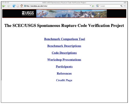
▲ Figure 3. Homepage of our SCEC/USGS code verification Web site. This page is available to all viewers and allows open access to information about the benchmarks, codes, and participants list. |
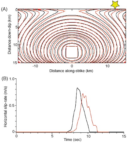
▲ Figure 5. Web page showing results for two spontaneous rupture codes that ran the TPV8 benchmark. One code is still in the developmental stage and so does not appear in the public section of the Web site; the other code is in the operational stage and does appear in the public section of the Web site. Comparisons show (A) the rupture-front contour plots that indicate where, at 0.5-s contoured intervals, the earthquake rupture first slipped the fault at ≥1 mm/s, and (B) the horizontal slip-rates in m/s at an on-fault station that is 12-km along strike from the epicenter. The station location is indicated by the star in A. Both the rupturefront contour plots and the synthetic seismograms qualitatively indicate a relatively poor match between these two codes. |
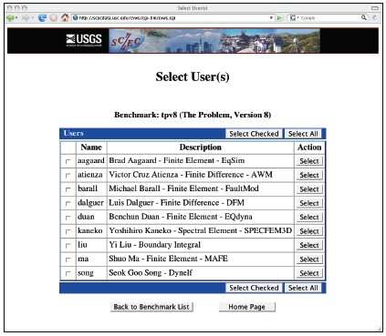 ▲ Figure 4. One of the code comparison Web pages. This public Web page lists the modelers and fully operational codes that performed the TPV8 benchmark. The specifications for this benchmark are outlined in Table 1 and provided in detail on the Web page http://scecdata.usc.edu/cvws/benchmark_descriptions.html. |
Our Web site (see Figure 3) lists our group’s participants, describes the code-verification benchmarks, and provides information about the codes that our participants are using. Modelers in our code comparison exercise upload their simulation results and view and compare all of the results that are produced by the codes in both developmental and operational stages. For each benchmark (starting with TPV5), the entire community can download the benchmark description, and, in the public section of the Web site, the entire community can compare the results of the fully operational codes that performed that benchmark. For example, Figure 4 lists the modelers and the fully operational codes that tackled the TPV8 benchmark (outlined in Table 1). The Web site can be used to compare the displacement, velocity, and stress time-histories generated by different codes at pre-assigned (in the benchmark description) seismic stations on or near the fault(s), at the Earth’s surface, and at depth. Early in our comparison exercise we found that contour plots of the earthquake rupture front, as the fault is just starting to slip (meet or exceed 1 mm/s slip-velocity) at each location on the fault, are quite diagnostic of overall similarity in code performance. That is, if the rupture-front contour plots generated by two different code simulations are not similar, then the synthetic seismograms generated by the two codes are also not going to match (Figure 5); the opposite also appears to be true, whereby matching contour plots indicate higher likelihood for good matching of synthetic seismograms (Figure 6). Therefore another verification test that we perform on the Web site is a comparison of the rupture-front contour plots.
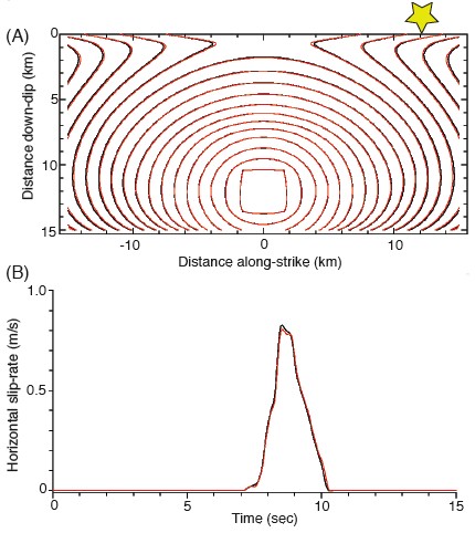
▲ Figure 6. Web page showing results for two fully operational spontaneous rupture codes that ran the TPV8 benchmark. Both codes appear in the public section of the Web site. Comparisons show (A) the rupture-front contour plots that indicate where, at 0.5-s contoured intervals, the earthquake rupture first slipped the fault at ≥1 mm/s, and (B) the horizontal slip-rates in m/s at an on-fault station that is 12-km along strike from the epicenter. The station location is indicated by the star in A. Both the rupturefront contour plots and the synthetic seismograms qualitatively indicate an excellent match between these two codes.
OVERVIEW OF OUR PROGRESS
Our code validation exercise started with simulations of ruptures on vertical strike-slip faults. This choice was dictated by ease of computation and to make sure that all of our participants’ 3D spontaneous rupture codes could perform these benchmarks. We also began with a simple friction formulation, slip-weakening, because almost all modelers have used this formulation in their research efforts and are therefore familiar with its implementation. There are, however, numerous dipping faults in the real world, so some of our benchmarks consider dipping fault scenarios. In addition we have also examined cases of more complex friction parameterizations.
Sometimes it seems as if the code validation exercise moves at a snail’s pace, but during the “down time” for some modelers, other modelers are improving their codes and finding bugs that they may have ignored in the past. One outcome is readily apparent. Without the code validation exercise there would surely have been earthquake rupture simulations, some of them highly visible research products, which were not done correctly. The SCEC/ USGS Rupture Dynamics Code Verification exercise is providing rigorous testing for the modelers and the codes involved.
FUTURE GOALS
Future goals for the code verification exercise include advances in calibration and verification measures. One immediate goal is to include quantitative comparison metrics. These metrics will help the SCEC/USGS Rupture Dynamics Code Verification project provide codes with a stamp of community approval. The convergence metric will allow modelers to determine if and when a specific code is producing results that are dependent on the discretization of the computational grid that comprises and surrounds the fault zone. Ideally, results should be grid-size independent. This type of convergence test has been performed by a few sets of modelers with a few codes (e.g. Day et al., 2005; Dalguer and Day 2007; Moczo et al., 2007; Kaneko et al., 2008), but has not to our knowledge been consistently featured among tests of numerous codes.
The misfit metric will serve to quantitatively assess intercode comparison, such as has been done by Moczo et al., 2007. Currently in the code-verification exercise we qualitatively judge if the results from multiple codes are in agreement, but a quantitative misfit measure would be more satisfactory. We envision that this misfit metric will assess the similarities and differences among the rupture-front contour plots and among the synthetic seismograms. The misfit metric will also assist us in our future comparisons of codes’ results and real data. A final goal for the code verification exercise is to move to that next step, that is, validation with field data. ![]()
| TABLE 1 Outline of Benchmark Specifications for TPV8 (see http://scecdata.usc.edu/cvws/benchmark_descriptions.html for full details) | ||
|---|---|---|
| Fault geometry | Vertical fault, top at earth’s surface | |
| Fault dimensions | 30-km-long × 15-km deep rectangle | |
| Material Properties | Homogeneous and linearly-elastic materials. Uniform Vp, Vs, density | |
| Initial shear stress direction | Along-strike | |
| Initial shear stress magnitude | Linear increase with depth | |
| Initial normal stress direction | Compressive | |
| Initial normal stress magnitude | Linear increase with depth | |
| Friction | Slip-weakening failure-criterion everywhere | |
| Nucleation-zone size | 3-km × 3-km rectangle | |
| Nucleation-zone location | centered at 15-km along-strike, 7.5-km along-dip | |
| Nucleation-method | Initial stresses set higher than yield stress | |
| Grid-spacing | 100 m | |
ACKNOWLEDGMENTS
Joe Andrews has thoughtfully contributed to our code comparison exercise in many ways, including by improving our benchmark descriptions. Funding for the Rupture Dynamics Code Verification Exercise has come from the Southern California Earthquake Center (funded by NSF Cooperative Agreements EAR-0106924, EAR-0529922, and USGS Cooperative Agreements 02HQAG0008, 07HQAG0008), internal USGS Earthquake Hazards Program funds, and the U.S. Department of Energy/Pacific Gas and Electric Extreme Ground Motions project. Thanks to Tom Jordan, Norm Abrahamson, Tom Hanks, and Paul Somerville for their support of this project, and thanks to Phil Maechling for graciously helping us with the logistics of the code-validation Web site. This manuscript benefited from helpful USGS internal reviews by Tom Hanks and Nick Beeler and from the comments of an anonymous SRL reviewer. This is SCEC Contribution #1184.
REFERENCES
Dalguer, L. A., and S. M. Day (2007). Staggered-grid split-node method for spontaneous rupture simulation. Journal of Geophysical Research 112, B02302; doi:10.1029/2006JB004467.
Day, S. M., L. A. Dalguer, N. Lapusta, and Y. Liu (2005). Comparison of finite difference and boundary integral solutions to three-dimensional spontaneous rupture. Journal of Geophysical Research 110, B12307; doi:10.1029/2005JB003813.
Dieterich, J. H. (2007). Applications of rate- and state-dependent friction to models of fault slip and earthquake occurrence. In Treatise on Geophysics, vol. 4, chapter 4, ed. H. Kanamori, 107–129. Amsterdam & Boston: Elsevier.
Harris, R. A. (2004). Numerical simulations of large earthquakes: Dynamic rupture propagation on heterogeneous faults. Pure and Applied Geophysics 161 (11/12), 2,171–2,181; doi:10.1007/s00024-004-2556-8.
Harris, R. A., and R. J. Archuleta (2004). Earthquake rupture dynamics: Comparing the numerical simulation methods. Eos, Transactions, American Geophysical Union 85 (34), 321.
Kaneko Y., N. Lapusta, and J.-P. Ampuero (2008). Spectral element modeling of spontaneous earthquake rupture on rate and state faults: Effect of velocity-strengthening friction at shallow depths, Journal of Geophysical Research, 113, B09317, doi:10.1029/2007JB005553.
Kostrov, B. V. (1964). Self-similar problems of propagation of shear cracks (tangential rupture crack propagation in medium under shearing stress). Journal of Applied Mathematics and Mechanics 28 (5), 1,077– 1,087.
Madariaga, R. (2007). Seismic source theory. In Treatise on Geophysics, vol. 4, chapter 2, ed. H. Kanamori, 59–82. Amsterdam & Boston: Elsevier.
Moczo, P., J. Kristek, M. Galis, P. Pazak, and M. Balazovjech (2007). The finite-difference and finite-element modeling of seismic wave propagation and earthquake motion. Acta Physica Slovaca 57 (2), 177–406.
Tullis, T. E. (2007). Friction of rock at earthquake slip rates. In Treatise on Geophysics, vol. 4, chapter 5, ed. H. Kanamori, 131–152. Amsterdam & Boston: Elsevier.
[ Back ]
Posted: 29 December 2008