
WebSims: A Web-based System for Storage, Visualization, and Dissemination of Earthquake Ground-motion Simulations
Kim B. Olsen
San Diego State University
Geoffrey Ely
University of Southern California
INTRODUCTION
Synthetic time histories from large-scale three-dimensional dynamic rupture or ground-motion simulations generally constitute large data sets, which typically require hundreds of megabytes, gigabytes or even terabytes of storage capacity (see, e.g., Olsen et al. 2008, 2009). For a seismologist analyzing rupture propagation or an earthquake engineer performing seismic hazard analysis, accessing large simulation output can be a tedious and error-prone procedure. For example, manual extractions of synthetic ground-motion records at a few sites of interest, or sliprate functions at desired locations on the fault, are subject to potential misinterpretation of site coordinates, units, or coordinate system orientation. If ground-motion synthetics or source-time functions are requested for a larger area (for example, to analyze site effects or rupture variability) additional problems may arise, such as bandwidth-related transfer delays, compatibility of storage devices used for dissemination, and time-consuming metadata assembly. Finally, the user may need to reformat the synthetics to apply post-processing steps, such as filtering or graphical display.
To circumvent these problems we have developed a userfriendly Web application (WebSims) that allows fast plotting, processing, storage, and dissemination of rupture and groundmotion simulations. WebSims allows interactive access to large multidimensional gridded synthetic data sets. Since there is a unique time history at each grid point for each scenario, static storage of plot images for each point would require extraordinary amounts of disk space. Thus, clearly, plots must be created dynamically. WebSims uses software that allows on-the-fly extraction and plotting of synthetic seismograms via a Web browser.
In terms of plotting and filtering features, but via different software, WebSims builds on a recent Web-based system used for validation of dynamic rupture simulations (Harris et al. 2009). However, an important difference from Harris et al.’s software is that WebSims is designed to manipulate large amounts of time series from simulations on a regular grid in a selected geographic area. WebSims also allows the option to simultaneously analyze the sliprate functions on the fault as well as the synthetic seismograms from the radiated waves. This option allows the user to interactively examine the source description for causes of amplification and other remarkable features in the ground-motion simulations. Another important application of WebSims is to facilitate verification of synthetic seismograms. For example, Bielak et al. (2009) compared ground velocities at selected sites for three different code bases, analyzing, among other features, the effects of anelastic attenuation, absorbing boundary effects, and media averaging. In the future, such analyses can be greatly facilitated by the availability of systems such as WebSims, which will eliminate the tedious manual handling, reformatting, and dissemination of synthetic time series after a series of simulations that may be required to understand the effects of various model parameters.
Description of WebSims
WebSims is accessed through a Web browser. The user selects an earthquake scenario from a searchable Matlab, which brings up maps of the fault and the area where sliprate histories and ground-motion synthetics, respectively, are available. We use maps of the rupture times, final slip, and peak sliprate distributions to locate the sliprate time histories, and a map of the peak ground velocities (PGVs) to locate the ground-motion histories. By clicking on an arbitrary site location, or by entering the site coordinates in an entry field, the corresponding time series are extracted from the underlying database of synthetics. The user has the option to lowpass filter (zero-phase, two-pole Butterworth) the selected time series to a desired bandwidth, a feature that can be useful in the presence of high-frequency numerical noise. WebSims also has the option to cross-plot time series from several scenarios at a desired site location, which allows the user to map differences in source (rupture time, peak sliprate, rise time, etc.) as well as ground-motion characteristics (arrival times, peak amplitudes, etc.). Below each time series plot, links are provided to download the raw time series data to the user’s local disk for further processing or analysis.
WebSims can also display two-dimensional maps (snapshots) of ground motion or sliprate. The time of the snapshot is selected by clicking the time axis of a time series plot or by using the entry field. The resulting snapshot image can, in turn, be used to pick a new time series location. In this way, the user can quickly move back and forth between the time (time series) and space (snapshots) domains using single mouse clicks.
Early versions of WebSims have been in the making since about 2003. WebSims1.0 used Hypertext Processor (PHP) to connect the synthetics in the database to the Web (Olsen and Martin 2003; Olsen and Talley 2006). At the time of this writing, the PHP interface was still in use to facilitate access to 7.3 terabytes of scenario simulations for large earthquakes on the southern San Andreas fault (TeraShake; Olsen et al. 2006, 2008) produced within the Southern California Earthquake Center (SCEC) at the San Diego Supercomputer Center (SDSC). However, WebSims Version 2.0 presented here uses a Python-based implementation. A clear advantage of Python for this type of application is the availability of free high-quality numerical, scientific, and graphical plug-in software packages. Python has a strong presence in scientific computing, competing with software such as MATLAB and Mathematica, while the strength of PHP is limited to Web programming. The switch from hand-coded PHP to Python (and supplemental mathematical and graphical packages NumPy (Dubois et al. 1996), SciPy (Jones et al. 2001), and MatPlotLib (Hunter 2007) in WebSims Version 2.0 roughly cut the number of lines of code in half (to about 1,000) while expanding the capabilities and improving the quality of the graphical output.
The availability of simulation metadata is essential for the use and interpretation of the seismic synthetics. For example, without information about orientation of axes, units, time spacing, projection, etc., analysis of the rupture process or the resulting ground motions is impossible. WebSims allows convenient storage and access to such metadata, directly linked to each simulation set.
The Web interface is implemented in strict HTML 4.01 without the use of JavaScript, Flash, cookies, or browser plug-ins. It is usable with older browsers (including the Lynx text-mode browser) with reduced functionality. In addition to the interactive Web interface, WebSims functions as a Web service, enabling machineto- machine communication and automated processing. The Web service is implemented in a representational state transfer (REST; Fielding 2000) style, where each resource (catalog search, plot, or data download) has a unique and permanent URL. The read-only REST design makes WebSims functionally equivalent to a collection of static Web pages. This promotes browser and proxy caching for increased performance and scalability. REST is simpler to implement and more natural for this type of data-centric Web service when compared to SOAP-based (Gudgin et al. 2007) solutions. The resource URLs are discoverable from the Web interface, which allows easy sharing among collaborators (for example) by copying and pasting URLs from the Web interface into e‑mail messages. The URL scheme is also useful for command-line utilities and scripting. Scripting is most convenient with Python because the native metadata format is valid Python syntax. Following retrieval from the Web service, metadata can be used directly by Python scripts, while use with other languages requires some amount of syntax parsing.
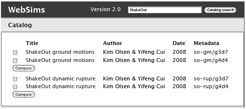
▲ Figure 1. Catalog page for WebSims, listing names, authors, date of ingestion, and location metadata, for the available (top) ground-motion scenarios and associated (bottom) source descriptions.
ILLUSTRATION OF WebSims
To illustrate how WebSims can facilitate scientific analysis, we have selected a subset of simulations of Mw 7.8 earthquakes on a 300-km by 16-km section of the southern San Andreas fault (SAF) performed for the Great Southern California ShakeOut exercise (Jones et al. 2008). Initial analysis of the ShakeOut simulations are presented by Graves et al. (2008, using kinematic source descriptions, “ShakeOut-K”) and Olsen et al. (2009, using spontaneous-rupture source descriptions, “ShakeOut-D”). Two different southeast-northwestward ShakeOut-D rupture scenarios (g3d7 and g4d4; Olsen et al. 2009), including sliprate time histories on the fault and associated ground-motion synthetics, have been ingested into WebSims Version 2.0 (see Figure 1). The source was modeled using spontaneous-rupture propagation on a mapped vertical approximation of the SAF, and the ground motions were obtained by inserting the resulting sliprate functions as a kinematic boundary condition on a segmented representation of the SAF (see Olsen et al. 2009 for further details of the two-step simulation procedure). Ground motions were calculated within an area 600 km by 300 km in southern California and northern Mexico using a finite-difference method (Olsen et al. 2009) and the SCEC Community Velocity Model version 4.0. The grid spacing of the rupture and ground-motion modeling was 200 m and 100 m, respectively. All time series are stored at a spacing of 200 m as four-byte floats in WebSims (1,501 (x) by 81 (y) by 625 (time) or 304 megabytes for each component of sliprate, and 3,000 (x) by 1,500 (y) by 625 (time) or 11.3 gigabytes for each component of ground velocities). While the storage required for the two scenarios (about 70 gigabytes) is not unreasonably large for numerical earthquake simulations, it is difficult to obtain an overview of the results without a user-friendly interface.
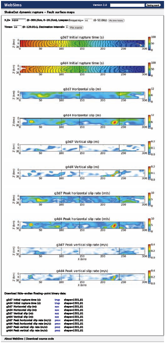
▲ Figure 2. Source descriptions used to illustrate WebSims (ShakeOut-D scenarios g3d7 and g4d4). Plots of the rupture time, horizontal and vertical slip distributions, and horizontal and vertical sliprates are displayed. At top, options are given for specifying the coordinates of the desired site location and low-pass filter cutoff frequency.
Figure 2 shows a display of rupture times, final (horizontal and vertical) slip, and peak (horizontal and vertical) sliprates for the g3d7 and g4d4 scenarios defined above from ShakeOut-D. These are plotted via the browser by checking the two available rupture scenarios and clicking “Compare” on the display in Figure 1. Similarly, Figure 3 shows a display of horizontal peak ground velocities (PGVs) along 130o and 40o clockwise from north for the ground motions resulting from the threedimensional wave propagation, plotted via the Web browser by checking the two available rupture scenarios and clicking “Compare” on the display in Figure 1. The vertical lines on the fault panels in Figure 2 depict boundaries of the four segments used in the ground-motion simulations, shown as black dots on the plots of the PGVs in Figure 3. Figure 4 shows a crossplot of the sliprate histories from scenarios g3d7 and g4d4 at a lateral distance from the left edge of the fault of 228.6 km and a depth of 9.8 km (see Figure 2). The site is selected inside a localized asperity for the g4d4 rupture scenario (toward the right end of the third fault segment from the left), which is absent for g3d7 (see Figure 2). The horizontal slip, sliprate, and slip acceleration for g4d4 at this site are about 12 m, 10 m/s and 20 m/s2, respectively, 5–23 times larger than the values for g3d7 at the same location. An area of large PGVs within a few kilometers of the fault (~ 390 km east, ~ 220 km north in Figure 3, bottom) is correlated with the localized asperity for g4d4. However, a similar area of large PGVs at the same location is found for g3d7. The most likely cause of the near-fault, localized amplification for g3d7 is the area of large horizontal slip (up to 8–9 m) between 230–245 km within the top 5 km of the fault for g3d7, without significant increase in the sliprate in this area (see Figure 2). Directivity effects from the southwestnortheastward rupture direction are likely the main reason why this area of large, shallow slip for g3d7 is displaced 10–30 km in the forward rupture direction, as opposed to the case for g4d4, where the largest PGVs are located immediately above the (deep) asperity. These observations demonstrate how a shallow area of moderate and gradual moment release can generate PGVs comparable to, or larger than, those for a strong and deep but spatially offset asperity.
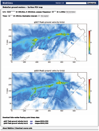
▲ Figure 3. Maps of the PGVs for the ground-motion scenarios, illustrated by the 600-km by 300-km ShakeOut-D models for sce-narios g3d7 and g4d4. At the top, options are given for speci-fying the coordinates of the desired site location and lowpass filter cutoff frequency.
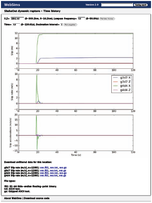
▲ Figure 4. Cross-plots of sliprates at a selected location on the fault.
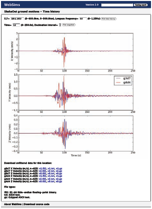
▲ Figure 5. Cross-plots of ground velocities at a selected location in the modeling area.
Figure 5 shows a cross-plot of the 130o and 40o components of ground velocities from scenarios g3d7 and g4d4 at a site near Santa Clarita (190.4 km, 146.0 km in Figure 3), interpreted to be inside a wave guide generating localized amplification. g3d7 shows an asperity of large slip (up to 7 m) and sliprate (6.5 m/s) between 40 km and 70 km (approximately in the middle of the leftmost fault segment), where g4d4 has a smaller asperity (20–25 km) but with larger slip (up to 7.5 m) and peak sliprate (up to 8.5 m/s). The near-fault area above the asperities for the two source descriptions shows more pronounced localized amplification for g3d7 than for g4d4 (see Figure 3), consistent with a larger moment release by g3d7 in this area. However, selected sites inside the wave guide show larger PGVs for g4d4 than for g3d7 (such as that shown in Figure 5). The result is likely due to the more abrupt release by g4d4 (larger peak sliprates and slip accelerations), radiating larger amounts of seismic energy into the wave guide.
Finally, note that both scenarios generate PGV distributions with “star burst” patterns from abrupt changes in the dynamic ruptures, as identified in Olsen et al. (2008) for the TeraShake simulations. However, the “star bursts” from g4d4 are much stronger than those from g3d7 due to larger sliprates and slip accelerations.
While plots of the synthetic time series are important, the associated metadata is essential for proper analysis and interpretation. WebSims is set up to store and list metadata for the source and ground-motions synthetics. Figure 6 shows the metadata for the g3d7 ground-motion scenario. The information includes the scenario name, authors, endian type, dimensions, axes, etc.
DISCUSSION AND FUTURE EXTENSIONS OF WebSims
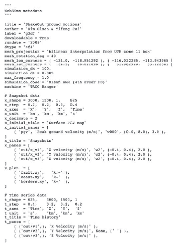
▲ Figure 6. Cross-plots of ground velocities at a selected location in the modeling area.
The features of WebSims Version 2.0 include storage as well as user-friendly and rapid plotting, processing, and dissemination of rupture and ground-motion simulations. It provides a convenient means of sharing synthetic time histories among researchers and earthquake engineers. We have illustrated WebSims Version 2.0 for two rupture and ground-motion simulations on the southern SAF and provided analysis of the results facilitated by the user-friendly access to comparison of rupture parameters, source-time functions, and PGVs.
A number of extensions can be added to improve the versatility of WebSims in the future. For example, access to real data can be added from strong-motion databases for validation of the ground-motions synthetics. An option to compute Fourier and/or response spectra from the ground-motion histories could be valuable for earthquake engineering applications. Finally, rather than time histories at individual selected sites, the extraction may be expanded to all sites within a specified area on the fault and/or ground surface.
Since our emphasis for WebSims Version 2.0 is on time series, the synthetics are stored with time as the fastest dimension, so that one time series can be extracted with a single contiguous read of the disk. Although bandwidth-dependent, extraction of time series for the ShakeOut-D scenarios generally require less than a second. When snapshot plotting is enabled, synthetics are typically reordered for contiguous access, with time as the slowest dimension. Contiguous access is critical for a scripted language such as Python where looping over multiple disk reads can incur a significant performance penalty. Multiple versions of the synthetics can coexist for both time series and snapshot access at the cost of increased storage. ![]()
ACKNOWLEDGMENTS
This work was supported by the Southern California Earthquake Center (SCEC) through National Science Foundation grants including: 1) Petascale Cyberfacility for Physics-based Seismic Hazard Analysis Research Project (PetaSHA) (EAR-0623704), and 2) Enabling Earthquake System Science through Petascale Calculations (PetaShake) (OCI-749313). This is SCEC publication #1312.
REFERENCES
Bielak, J., R. W. Graves, K. B. Olsen, R. Taborda, L. Ramirez-Guzman, S. M. Day, G. Ely, D. Roten, T. H. Jordan, P. Maechling, J. Urbanic, Y. Cui, and G. Juve (2009). The ShakeOut earthquake scenario: Verification of three simulation sets, in revision.
Dubois, P. F., K. Hinzen, and J. Hugunin (1996). Numerical Python. Computers in Physics 10 (3), 262–267.
Fielding, R.T. (2000). Architectural styles and the design of network-based software architectures. PhD diss., University of California, Irvine; http://www.ics.uci.edu/~fielding/pubs/dissertation/top.htm.
Graves, R. W., B. Aagaard, K. Hudnut, L. Star, J. Stewart, and T. H. Jordan (2008). Broadband simulations for Mw 7.8 southern San Andreas earthquakes: Ground motion sensitivity to rupture speed. Geophysical Research Letters 35, L22302; doi:10.1029/2008GL035750.
Gudgin, M., M. Hadley, N. Mendelsohn, J. Moreau, H. F. Nielsen, A. Karmarkar, and Y. Lafon (2007). SOAP Version 1.2. Part 1: Messaging framework. 2nd ed., World Wide Web Consortium; http://www.w3.org/TR/soap12-part1/.
Harris, R. A., M. Barall, R. Archuleta, E. Dunham, B. Aagaard, J. P. Ampuero, H. Bhat, V. Cruz-Atienza, L. Dalguer, P. Dawson, S. Day, B. Duan, G. Ely, Y., Kaneko, Y. Kase, N. Lapusta, Y. Liu, S. Ma, D. Oglesby, K. Olsen, A. Pitarka, S. Song, and E. Templeton (2008). The SCEC/USGS dynamic earthquake-rupture code verification exercise. Seismological Research Letters 80 (1), 119–126; doi:10.1785/gssrl.80.6.119.
Hunter, J. D. (2007). Matplotlib: A 2D graphics environment. Computing in Science and Engineering 3 (9), 90–95.
Olsen, K. B., S. M. Day, L. Dalguer, J. Mayhew, Y. Cui, J. Zhu, V. M. Cruz-Atienza, D. Roten, P. Maechling, T. H. Jordan, and A. Chourasia (2009). ShakeOut-D: Ground motion estimates using an ensemble of large earthquakes on the southern San Andreas fault with spontaneous rupture propagation. Geophysical Research Letters 36, L04303; doi:10.1029/2008GL036832.
Olsen, K. B., S. M. Day, J. B. Minster, Y. Cui, A. Chourasia, M. Faerman, R. Moore, P. Maechling, and T. Jordan (2006). Strong shaking in Los Angeles expected from southern San Andreas earthquake. Geophysical Research Letters 33, L07305; doi:10.1029/2005GL025472.
Olsen, K. B., S. M. Day, J. B. Minster, Y. Cui, A. Chourasia, R. Moore, P. Maechling, and T. Jordan (2008). TeraShake2: Simulation of Mw 7.7 earthquakes on the southern San Andreas fault with spontaneous rupture description. Bulletin of the Seismological Society of America 98, 1,162–1,185; doi:10.1785/0120070148.
Olsen, K. B., and A. Martin (2003). Websim3d: A web-based system for generation, storage and dissemination of earthquake ground motion simulations. Eos, Transactions, American Geophysical Union 84 (46), Fall Meeting Supplement ED32C-1206.
Olsen, K. B., and J. Talley (2006). User interface for cross-plot, filtering and upload/download of timeseries. In Proceedings of the Annual SCEC Meeting, Palm Springs, CA, 9–14 Sept., p. 138. Los Angeles: Southern California Earthquake Center.
[ Back ]
Posted: 22 October 2009