Hiller’s Seismoscope

doi:10.1785/gssrl.81.5.804

Klaus-G. Hinzen¹ and Roman Kovalev²

Click to Show (or Hide) Authors' Affiliations

1. Earthquake Geology Group, Institute for Geology and Mineralogy, University of Cologne, Bergisch Gladbach, Germany
2. Laboratory of Computational Mechanics, Bryansk State Technical University, Bryansk, Russia

INTRODUCTION

Seismoscopes had already existed for a while before the first expedient seismometers were constructed at the end of the 18th century. The most famous one, which every undergraduate student of geosciences knows, is Zang Hêng’s (also referred to as Chôko and Tyoko “didongy” (earth movement instrument) of A.D. 132 (Dewey and Byerly 1969). An educational summary of early seismological instrumentation can be found at http://earthquake.usgs.gov/learn/topics/seismology/history/history.

It was not until the 19th century that real new developments of seismoscopes were made. Among seismologists experimenting with seismoscopes was Wilhelm Hiller (Figure 1). After studying mathematics and physics, at the age of 24 Hiller joined the Meteorologische Abteilung des Statistischen Landesamtes, also called Württembergische Erdbebenwarte (Seismological Observatory of Württemberg). His early studies concentrated on surface wave analysis, which also became the theme of his Ph.D. thesis at the Technical University Stuttgart in 1926 (http://www.dgg-online.de/geschichte/seiten_htm/dgg_136.htm). In 1929 the opportunity arose for him to modernize this seismological observatory, and he moved it from Hohenheim to the Villa Reitzenstein in Stuttgart. There he set up one of the most sophisticated seismological stations of his time. He installed seismographs of different types with a wide range of amplitudes and frequencies. After the second World War, Hiller worked intensively in the field of seismometry. Among other instruments, he created a seismometer named “Type Stuttgart” for local seismic measurements (Figure 1). More than a hundred sets of these were built by the Feinwerkschule Schwenningen (a school for fine mechanics). In 1961 the U.S. Coast and Geodetic Survey assigned Hiller the only World-Wide Standard Seismograph Network (WWSSN) station in Germany, which was operational until 1990 (http://www.dgg-online.de).

(A)

(B)

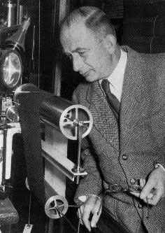
▲ Figure 1. A) Wilhelm Hiller (1899–1980) (http://www.dgg-online.de). B) Horizontal seismometer “Type Stuttgart” for local and regional earthquakes developed by Hiller and built by Feinwerkschule Schwenningen.

Even after the advent of usable seismometers, interest in and development of seismoscopes did not stop. In the 1930s Hiller was among the pioneers of earthquake fault plane solution. He intended to increase the number of P-wave first motion observations by using a simple instrument, the Stossrichtungsanzeiger nach W. Hiller (Figure 2). The German name, which translates to “direction of impact detector,” indicates that the main purpose was the measurement of the (first) ground motion direction and not earthquake detection. For ease of reading, we will hereafter refer to this as “Hiller’s seismoscope.”

After the 1951 Euskirchen (M_S 5.2) earthquake damaged parts of the Lower Rhine embayment (Schwarzbach 1951; Hinzen and Reamer 2007), Cologne University founded the seismological station Bensberg on 25 August 1951. The initiative came from Martin Schwarzbach, head of the university’s Geological Institute. Schwarzbach, a geologist, did not have the necessary expertise to establish a seismological station, and so Hiller and his assistants became responsible for establishing the new station in the Rhineland.

(A)

(B)

(C)

COMPUTER MODEL

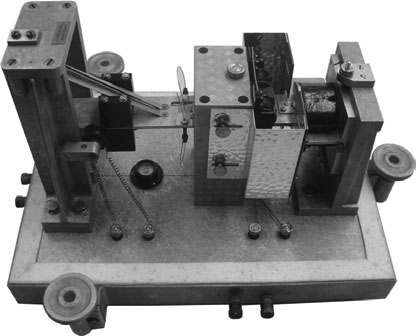
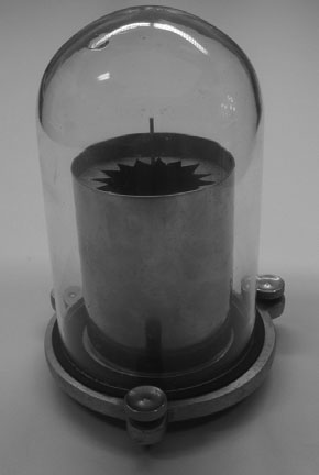
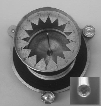
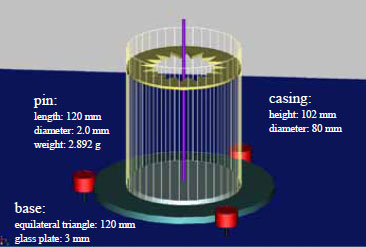
Figure 2 shows a photo of Hiller’s seismoscope (item on loan from the Black Forest Observatory, BFO). The three feet of the base plate are arranged at the corners of an equilateral triangle with sides 120 mm long. Two of the feet are height-adjustable for leveling; however, the instrument does not have a built-in bubble level or anything similar. The base plate sits on top of the casing cylinder, which is 80 mm in diameter and 102 mm high. At a height of 87 mm measured from the base plate is a “star” with 16 triangular slots corresponding to a resolution of 22.5° of the toppling direction of a pin at the center of the instrument. The slots are numbered clockwise from 1 to 16 with numbers 8 and 16 in line with one of the adjustable feet. In the computer model (Figure 3) of the instrument (described later) this direction was chosen as the x-axis, with the positive direction pointing toward the foot. Directly on the base plate, inside the casing cylinder, sits a loose glass plate that fits tightly into the circumference of the cylinder with a thickness of 3 mm. The active part of the instrument, the toppling pin, is a steel cylinder 120 mm high and 2 mm in diameter. This is placed manually in the center of the glass plate. The bottom of the pin has a coneshaped concavity to make sure it rests on its outer circumference (Figure 2C). The weight of the pin is 2.89 g, and it takes a steady hand to set it up. Hiller, who could set up the pin in a few seconds, reportedly enjoyed teasing his assistants (some of whom later became very well known seismologists: Hans Berckhemer, Stephan Müller, Goetz Schneider, Rolf Schick, Walter Zürn), who sometimes needed several minutes to successfully arm the instrument (R. Schick, personal communication, 2010).

▲ Figure 3. Perspective view of the discrete elements of the numerical model used in this study. Measurements were taken from the original instrument.

A computer model of Hiller’s seismoscope was developed and analyzed with the help of the general-purpose multibody code “Universal Mechanism” (UM) (Pogorelov 1995, 1997). As typical multibody software, UM is based on classical theory, automatically derives equations of motion of mechanical systems, and uses numerical methods to solve these equations in the time domain. Multibody system dynamics is a part of classical mechanics that is devoted to computer-oriented methods and their applications. One of the most detailed surveys of multibody dynamics, including modeling analysis methods and applications, was presented by Schiehlen (1997). UM uses an approach of nondeformable 3D objects with small overlaps at the points of contact (Kraus et al. 1997). In the computer model the parameters of the coupling forces between the pin and the glass plate were set according to the materials in contact. The dynamic coefficient of friction in the model was set to 0.5, and 0.6 was set for the static friction coefficient (http://www.engineershandbook.com/Tables/frictioncoefficients.htm). The contact frequency was 200 Hz in all experiments and the damping ratio of the coupling was 0.3.

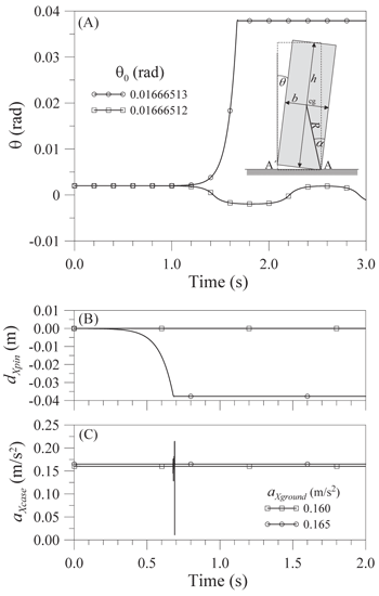
▲ Figure 4. Results of two tests of correct model behavior. A) Rotation angle θ of the pin in a free motion with two different initial inclinations, θ₀, slightly above and below the indifferent equilibrium. The inset shows the parameters of the rocking block mentioned in the text. B) Displacement of the pin, d_Xpin, at a height of 87 mm in x-direction and C) acceleration of the instrument case, a_Xcase, for two levels of constant ground acceleration. The spike in the a_Xcase signal at 0.165 m/s2 acceleration results from the falling pin hitting the case.

Model Verifications

In order to test the correct behavior of the numerical UM model, we performed two tests, one observing the free motion of the pin following varied initial static inclinations and one with constant ground acceleration. We then compared the results of both numerical experiments with the analytic solutions for these simple tests.

The free rocking motion of a rectangular block, similar to the cylinder in a 2D experiment, was given by Housner (1963), who studied overturned objects after the famous 1960 Chile earthquake. When a rectangular block of height h and width b is turned over one of its corners A (Figure 4A), and initial velocities of the ground and the block are zero, it will fall back to its equilibrium position after a rocking motion if the inclination angle θ is smaller than α, the angle between the vertical direction and the line connecting the center of gravity with the rocking corner A; if θ is larger than α, the block will turn over. The critical angle in the case of Hiller’s seismoscope is arctan(b/h) = 0.16 rad. Figure 4A shows the time history of the rotation angle θ of the toppling pin around the y-axis for two initial inclinations, θ0. In one case the initial inclination is smaller than α in the 8th digit when measured in radians, and in the other it exceeds α in the 8th digit. The initial velocity is always set to zero. As predicted by theory, in the first case the pin returns to its equilibrium after a rocking motion, while in the second case it overturns and comes to a rest in the expected slot of the instrument’s star number 8 (Figure 4).

The second test was one with a forced movement. Housner (1963) gave the yield constant horizontal acceleration necessary to overturn a rectangular block. Considering the pin of the instrument this acceleration is 0.163 m/s². Figure 4B shows the pin movement in the x-direction measured at the height of the catching star for horizontal accelerations of 0.160 m/s² and 0.165 m/s², values slightly below and above the predicted threshold. These two cases produce the expected results. The spike in the acceleration record of the instrument’s case at 0.68 s in Figure 4C results from the falling pin striking the case.

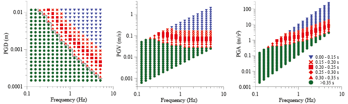
▲ Figure 5. Result of a sensitivity test of Hiller’s seismoscope with ground motion of damped sinusoidal pulses in the x-direction. The symbols in the plot give the time between the start of the experiment and when the pin hits the case. Round green symbols indicate that the pin did not fall. The black step plot separates the experiments with fallen and not fallen pin. From left to right the maximum displacement (PGD), velocity (PGV), and acceleration (PGA) of the damped sinusoidal pulses are given.

SENSITIVITY TO IMPULSIVE MOTION

We tested the sensitivity of the instrument to horizontal ground motions with a set of damped sinusoidal impulses. The damping ratio was chosen as 12:1 and the amplitude and frequency range of impulses covered 1 × 10⁻⁴ m to 1 × 10⁻² m and 0.125 to 5 Hz. Both displacement amplitude and the frequency were increased in equally sized steps on a logarithmic scale. The results of the set of 340 numerical experiments are summarized in Figure 5. The times indicated in the plot are those from the start of the ground motion until the pin hits the slot of the star. The ground was kept at rest for 0.1 s in all calculations before the onset of the ground motion to ensure that any minor static settlements in the model had taken place before the ground motion started. The round symbols in Figure 5 indicate that the pin did not topple. The impulse with the largest acceleration amplitude at a frequency of 5 Hz and displacement 2 × 10⁻² m leads to the shortest falling time, as expected. With decreasing peak acceleration the falling time increases until a threshold is reached beyond which the pin does not fall; this threshold is indicated in Figure 5 by the step line. In a frequency range from 0.5 to 5 Hz, suitable for the local earthquakes targeted by Hiller’s experiments, the threshold of peak ground displacement amplitude of a damped sinusoidal impulse decreases from 0.01 to 0.0002 m. Between 0.2 and 1 Hz, the PGV threshold decreases from 0.07 to 0.03 m/s, and for frequencies above 1.25 Hz the threshold is constant at 2.8 mm/s. The PGA threshold increases from 0.36 m/s² at 0.2 Hz to 3.3 m/s² at 5 Hz.

We studied the effect of an imperfect leveling of the instrument in six additional sets of calculations. It was assumed that the foot in the +x-direction (Figure 3) shows maladjustments of +0.5, +0.25, +0.1, −0.1, −0.25, and −0.5 mm, which corresponds to an inclination of the base plate of ±9.6 × 10⁻⁴ to ±4.8 × 10⁻³ rad. Figure 6 shows that for a ±0.1-mm maladjustment the instrument’s behavior is unchanged. At the 0.25-mm level, raising the foot slightly increases the sensitivity at the high-frequency end of the tested parameter space. Lowering the foot has the opposite effect at lower frequencies. As the first ground motion is always in the positive x-direction, the pin in this case has to be moved further during the tests than in the case of a perfect leveling. At a maladjustment of ±0.5 mm the effects become stronger, but the falling direction was always the expected one. However, even though the instrument does not carry a built-in level, a leveling within the ±0.25-mm range (or better) is easily achieved with a leveling device placed on the case during installation. Based on these analyses, we concluded that a small maladjustment of the instrument does not alter the results obtained by the instrument.

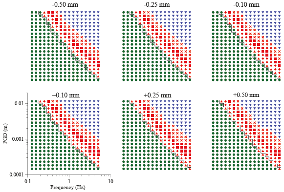
▲ Figure 6. The six plots show the influence of deviations of a perfect leveling of the Hiller seismoscope on its sensitivity. The numbers given above each plot give the heights of the deviation of the instrument’s foot, which is in alignment with the x-axis parallel to the direction of motion. The black step line indicates the sensitivity of the perfectly leveled instrument.

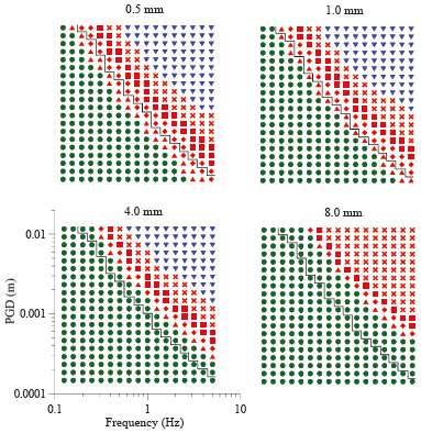
▲ Figure 7. Four plots showing the sensitivity of Hiller’s Seismoscope to the same ground motions as those used in Figure 5 for assumed diameter on the pin of 0.5, 1.0, 4.0, and 8.0 mm. The black step line indicates the sensitivity of the original instrument with a 2-mm diameter pin for comparison (see Figure 5).

The numerical model also allowed a study of the instrument sensitivity after posing the question: what if Hiller had chosen another dimension of the pin? We used pins with a fourth, half, double, and quadruple the nominal diameter of 2 mm. The results of the single component excitation tests are shown in the four panels of Figure 7. The increased and decreased sensitivity in cases of smaller and larger pin diameters, respectively, is obvious in the entire tested frequency range. On average over the tested frequency range, the increase in displacement sensitivity for the 1.0 and 0.5 mm pins are 1.7 and 3.0 fold; the decrease in cases of the 4.0 and 8.0 mm pins is 2.5 and 5.5, respectively.

The seismic station in Stuttgart still owns a seismoscope built by Galitzin, which was probably purchased in 1914. This instrument is equipped with nine pins of different diameters. It has a simple octagon as the catching device, indicating that Galitzin’s goal with this instrument was for simple detection and not for the determination of source direction. The radiation pattern of a point source with shear mechanism was not published until Honda (1934).

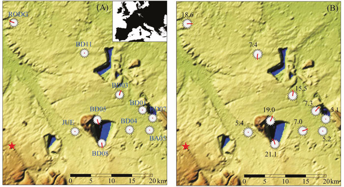
▲ Figure 8. The maps show the location of the 22 June 2002 Alsdorf earthquake (M_L 4.9) in the Lower Rhine Embayment and 10 shortperiod stations at distances between 15 and 35 km. At each station location the 16-notch star from Hiller’s Seismoscope is plotted and in red the track of the pin of the instrument from the equilibrium position to its final resting position is shown. Maps (A) and (B) show the results for a 2- and 1-mm diameter pin, respectively, and station codes and peak ground accelerations in cm/s². The geometric features in the digital elevation model are large open lignite mines. The inset in the upper right corner of map (A) indicates the map location within Europe.

Local Earthquake

The measured ground motions of a local earthquake that occurred in the Lower Rhine embayment on 22 July 2002 with its epicenter close to the city of Alsdorf (Figure 8) M_L = 4.9 (Hinzen 2005) were used to calculate the performance of Hiller’s seismoscope under “field conditions.” The event was located at a depth of 15.8 km. Ten stations of the Cologne University network (http://www.seismo.uni-koeln.de) were located at epicentral distances between 21 and 35 km (Figure 8). The velocity-proportional seismograms of these stations were integrated and the 3D ground displacements in the frequency range from 0.8 Hz to 20 Hz were used as an input time signal. The pin toppled at four of the 10 stations. At these locations the maximum acceleration exceeded 15 cm/s² while peak ground acceleration (PGA) did not reach 10 mm/s² at the other six stations. This threshold of PGA during the realistic ground motion is lower than that derived from the one-component sinusoidal impulse tests (Figure 5). This is due both to the combined motion in three dimensions and the reverberations at the softrock stations.

The path of the pin at a level of 87 mm above the base, where it hits the star if it falls, is shown in Figure 9 in detail for the four stations where the pin fell. At the first hit of the pin on the star it changes its direction and more or less slides along the star until it comes to rest in one of the pointed slots. The triangular slots corresponding to the radial direction of wave spreading are indicated in Figure 9. The toppling direction at stations BD05 and BD08 is four slots clockwise with respect to the radial direction, which, taking the 22.5° resolution into account, agrees with the transverse direction. At station RODG the toppling is three slots counterclockwise from the radial direction. While for these three stations the toppling direction agrees with the transverse (SH) wave motion, at station BD03 the pin falls two slots counterclockwise from the radial direction, right in between the radial and transverse direction. Also in these cases, the late toppling times observed in the numerical tests indicate that the P-pulse was not sufficiently large to overthrow the pin.

In a further test, we assumed that Hiller’s Seismoscope, when recording the Alsdorf earthquake, was equipped with a 1-mm diameter pin (Figure 8B). Among the ten stations the pin toppled at an additional three stations with PGAs between 7 cm/s² and 10 cm/s². At stations RODG, BD05, and BD08 the toppling direction of the 1-mm pin is nearly opposite that of the 2-mm pin.

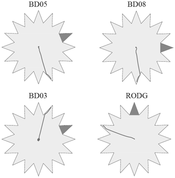
▲ Figure 9. Details of the movement of the toppling pin of Hiller’s Seismoscope at four local seismic stations (see Figure 8 for locations) during the Alsdorf 2002 earthquake from results of a numerical test. Shown is a top view of each instrument and the path of the falling pin at a height of 87 mm. The shaded triangles indicate the sections that correspond to the positive radial directions with respect to the earthquake location.

DISCUSSION AND CONCLUSIONS

We tested the performance of a simple seismoscope designed by Wilhelm Hiller with a numerical model of the instrument. The name “Stossrichtungsanzeiger” used by Hiller indicates that the direction of the ground motion was the focus of the deployment of instruments in the Swabian Jura in the 1930s rather than just the detection of events. The idea of using a large number of these simple instruments to collect enough P polarities for fault plane solutions is self-evident. However, one main disadvantage of the instrument in this respect is that there is no way to determine during which part of the ground motion in an earthquake toppled the pin.

We can show that in a frequency range from 0.2 to 5 Hz, suitable for the targeted local earthquakes, the threshold of peak ground displacement amplitude of a damped sinusoidal impulse decreases from 0.01 to 0.0002 m. Between 0.2 and 1 Hz, the peak ground velocity (PGV) threshold decreases from 0.07 to 0.03 m/s, and for frequencies above 1.25 Hz the threshold is constant at 2.8 mm/s. PGA threshold increases from 0.36 m/s² at 0.2 Hz to 3.3 m/s² at 5 Hz.

The instrument is not equipped with a built-in bubble level; however, small deviations from vertical, well within the range which is in practice achievable in the field from a perfectly leveled state, do not alter the sensitivity significantly.

The test with measured ground motions from a local M_L 4.9 earthquake shows that the toppling directions resemble more the transverse (SH) ground motion than the P-wave polarity. In this respect, the instrument does not provide reliable measures for the construction of fault plane solutions. Hiller himself wondered that the pin might “tremble a little” before toppling and that there was no guarantee that Pn or Pg phase or later phases, especially S, would not “first” throw the pin (Schick, personal communication, 2010).   

REFERENCES

Dewey, J., and P. Byerly (1959). The early history of seismometry (to 1900). Bulletin of the Seismological Society of America 59, 183–227.

Hinzen, K.-G. (2005). Ground motion parameters of the 22 July 2002 M_L 4.9 Alsdorf (Germany) earthquake. Bolletino di Geofisica 46, 303–318. In English.

Hinzen, K.-G., and S. K. Reamer ( 2007). Seismicity, seismotectonics, and seismic hazard in the northern Rhine area. In, Continental Intraplate Earthquakes: Science, Hazard, and Policy Issues, ed. S. Stein and S. Mazzotti, 225–242. Geological Society of America Special Paper 425. Boulder, CO: Geological Society of America.

Honda, H. ( 1934). On the amplitudes of the P and S waves of deep earthquakes. Geophysical Magazine, Tokyo 8, 153–164.

Housner, W.G. (1963). The behavior of inverted pendulum structures during earthquakes. Bulletin of the Seismological Society of America 53, 403–417.

Kraus, P. R., A. Fredriksson, and V. Kumar (1997). Modeling of frictional contacts for dynamic simulation. In Proceedings of International Conference on Intelligent Robots and Systems (IROS) Workshop on Dynamic Simulation: Methods and Applications 1997 IEEE/ RSJ International Symposium on Robotic and Intelligent Systems Grenoble, France, 33–38.

Pogorelov D. Y. (1995). Numerical modeling of the motion of systems of solids. Computational Mathematics and Mathematical Physics 4, 501–506.

Pogorelov D. Y. (1997). Some developments in computational techniques in modeling advanced mechanical systems. In Proceedings of IUTAM Symposium on Interaction between Dynamics and Control in Advanced Mechanical Systems, e d. D . H . v an C ampen, 3 13– 320. Eindhoven, the Netherlands, 21–26 April 1996. Dordrecht: Kluwer Academic Publishers.

Schwarzbach, M. (1951). Erdbeben des Rheinlandes. Kölner Geologische Hefte 1, 3–28. In German.

Schiehlen W. (1997). Multibody system dynamics: Roots and perspectives. Multibody System Dynamics 1, 149–188.

Earthquake Geology Group Institute for Geology and Mineralogy University of Cologne Vinzenz-Pallotti-Str. 26 D-51429 Bergisch Gladbach, Germany hinzen [at] uni-koeln [dot] de (K.-G. H.)