This supplemental information includes five figures and two tables. The figures contribute supporting information for discussion in the main article, including complete model residuals and Coulomb stress analysis. Table S1 is a data table of continuous and campaign Global Positioning System (GPS) displacements used in this study. Table S2 describes the fault model parameters.
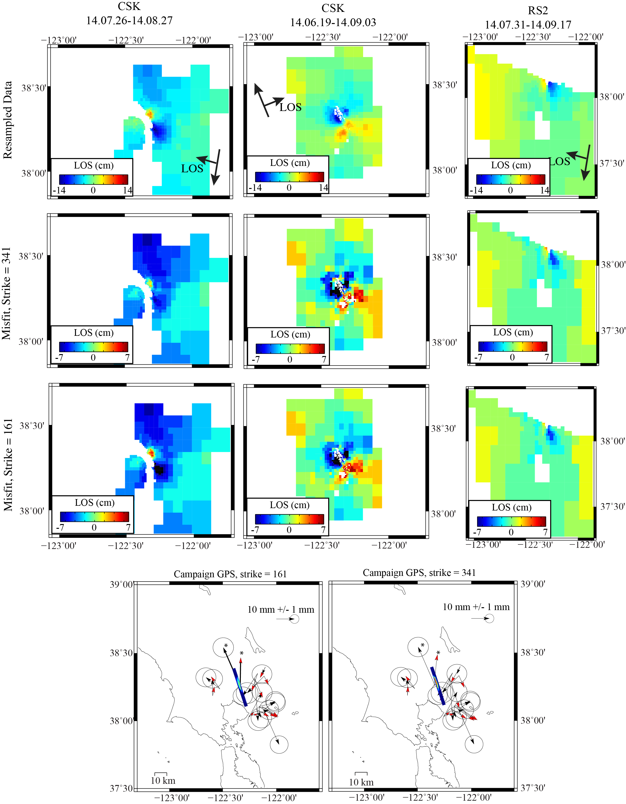
Figure S1. Interferometric Synthetic Aperture Radar (InSAR) and campaign GPS observations and model residuals for the slip distributions shown in Figure 2 in the main article. InSAR observations show the resampled observations and (data-predicted) model residuals. The campaign GPS horizontal observations (black) and predicted displacements (red) are both shown. Vectors marked with asterisks have been downscaled by a factor of ten for the purposes of display. Continuous GPS observations and model fits are shown in Figure 2. All continuous and campaign GPS observations are available in Table S2. Vectors on the InSAR displacement panels indicate the satellite azimuth and line of sight (LOS) direction. Note the difference in color ranges of displacements and residuals.
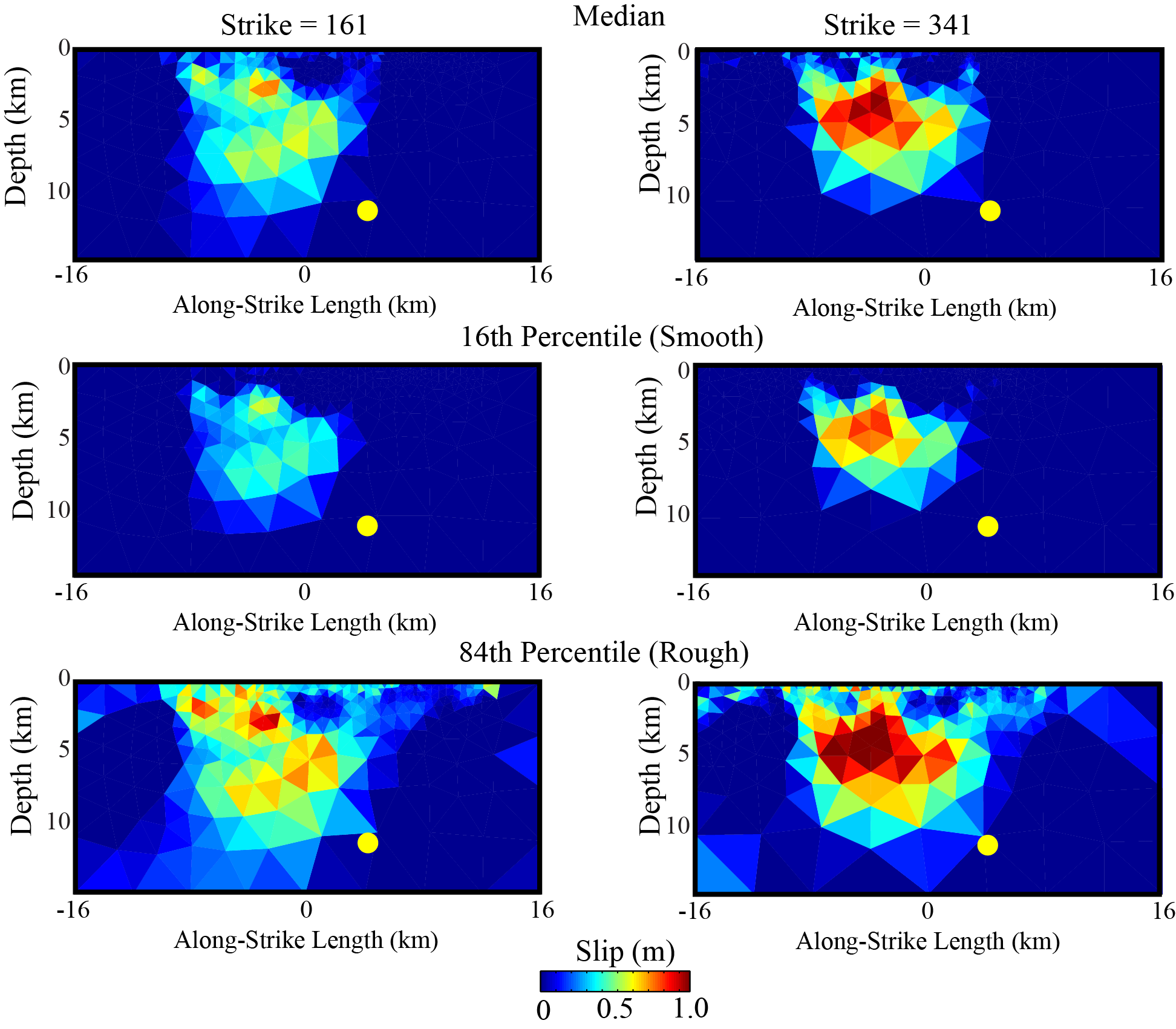
Figure S2. Slip distributions for the South Napa earthquake, derived from Monte Carlo analysis (left column, west dipping; right column, east dipping). The median slip distributions are the same as those shown in Figure 2 in the main article, and the 16th and 84th percentile slip distributions are shown for comparison. All slip distributions are plotted on the same color scale. Yellow dots indicate the location of the U.S. Geological Survey hypocenter (122.312° W, 38.215° N, 11.3 km).
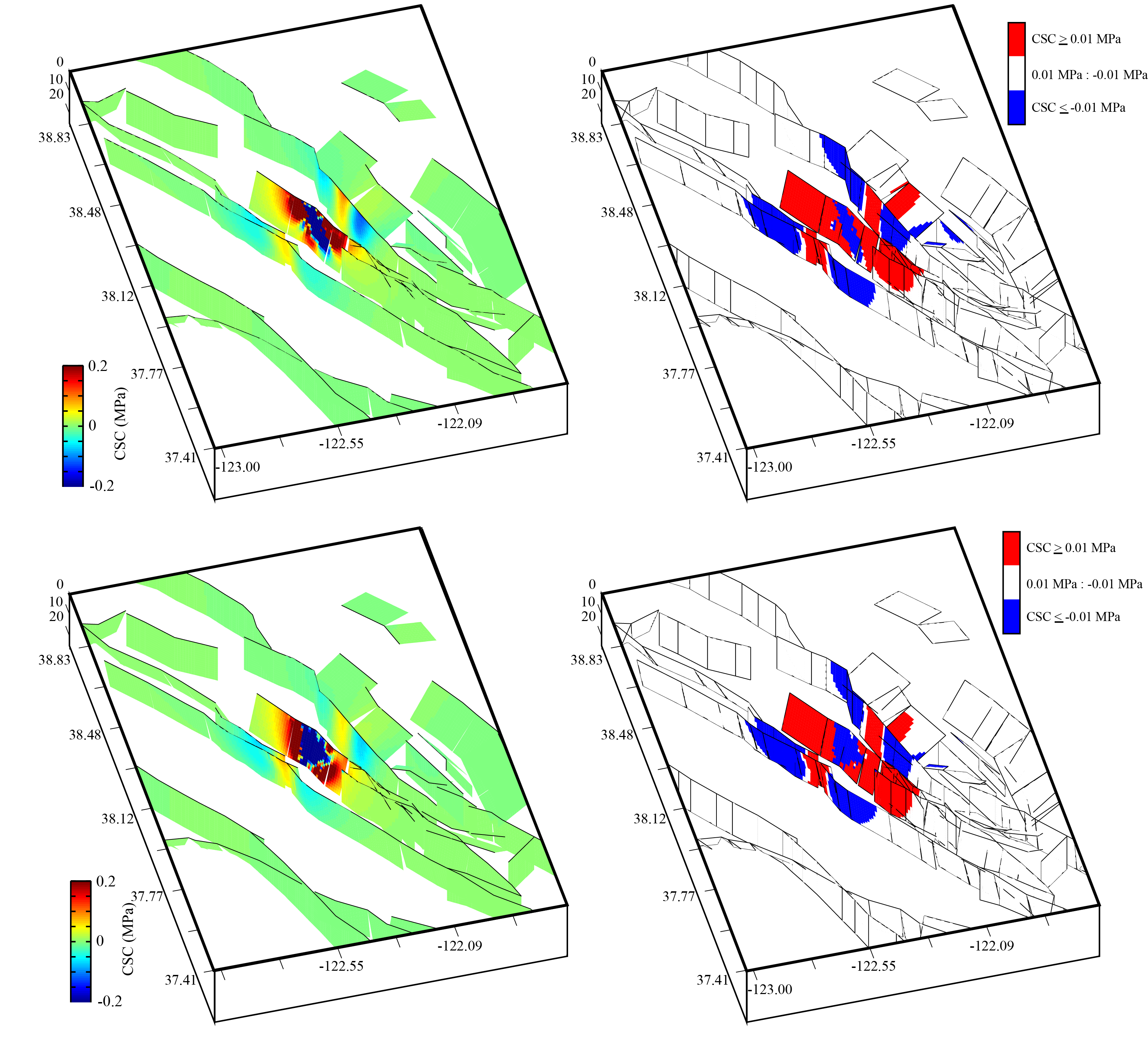
Figure S3. Predicted Coulomb stress changes, assuming a coefficient of friction of 0 on the receiver faults. As in Figure 4 of the main article, black traces indicate the tops of faults; red and blue regions indicate where the fault stress exceeds ±0.01 MPa threshold, with red indicating stress increase and blue indicating stress decrease; and white regions indicate stress changes between 0.01 and −0.01 MPa. Stress changes are resolved into the slip direction of each fault (e.g., Field et al., 2014, is mentioned for similar material in the caption for Figure 4 in the main article) .
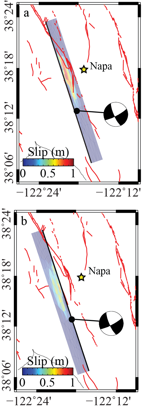
Figure S4. Enhanced view of the South Napa earthquake slip distribution with respect to local mapped faults. The surface trace of both faults is located west of the mapped faults (red, USGS Quaternary fault database, http://earthquake.usgs.gov/hazards/qfaults/; last accessed January 2015), in agreement with preliminary field observations. (a) Plane is striking 341°. (b) Plane is striking 161°.
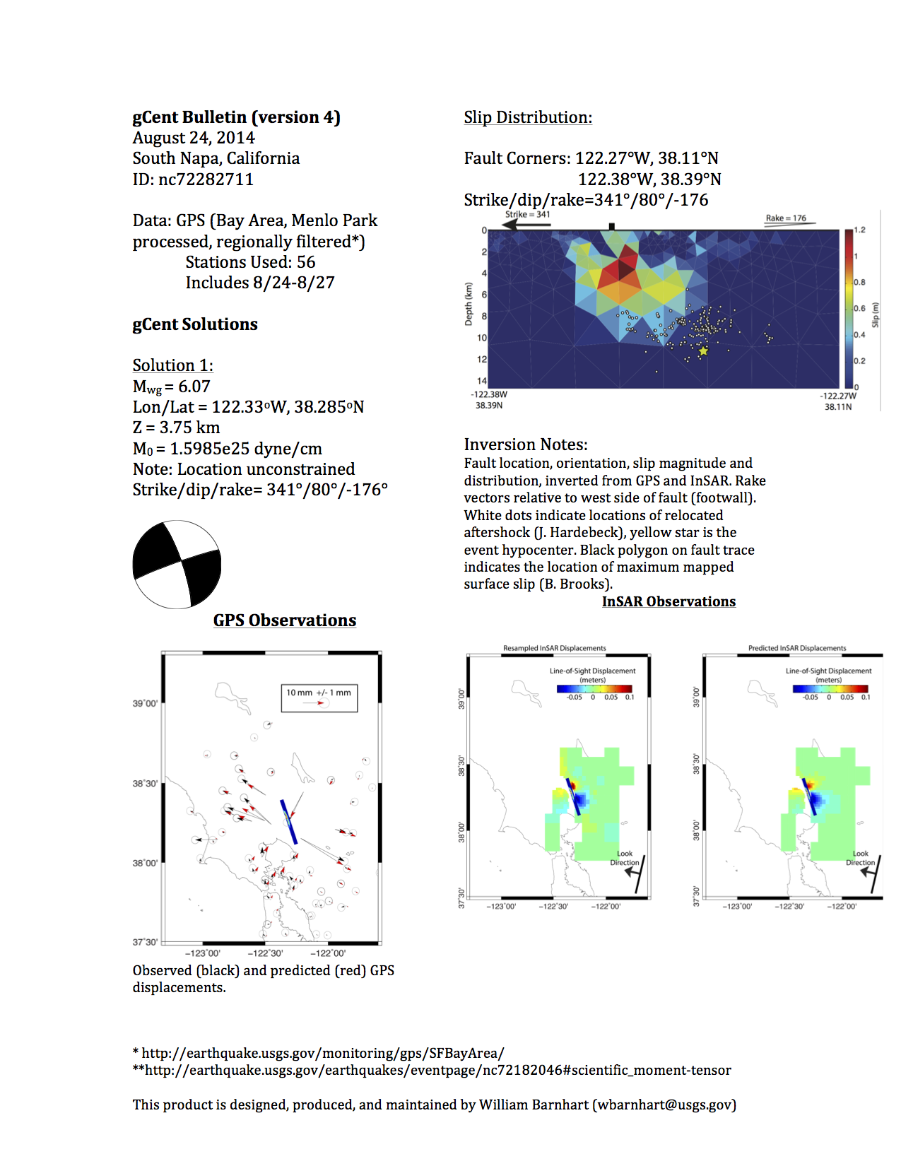
Figure S5. Example of the Geodetic Centroid Bulletin (gCent Bulletin) that was distributed internally within the USGS describing geodetic modeling of the South Napa earthquake. The example shown was the third released version, on 1 September 2014 (origin time + 7 days), which included continuous GPS observations and the descending COSMO–SkyMed (CSK) interferogram (e.g., Field et al., 2014, is mentioned for similar material in the caption for Figure 4 in the main article).
Table S1. Continuous and campaign GPS displacements used in this study. All units (except longitude and latitude) are in meters. Continuous GPS displacements include up to three days of postseismic deformation. ID indicates the continuous station identification code.
Table S2. Fault geometry and orientation derived from the neighborhood algorithm for each possible focal plane. These geometries are then used in geometries for distributed slip. Strike, dip, and rake are derived by the neighborhood algorithm. X0/Y0 indicate the top corner of the fault plane from the base of the strike direction.
Field, E. H., R. J. Arrowsmith, G. P. Biasi, P. Bird, T. E. Dawson, K. R. Felzer, D. D. Jackson, K. M. Johnson, T. H. Jordan, C. Madden, et al. (2014). Uniform California Earthquake Rupture Forecast, version 3 (UCERF3)—The time-independent model, Bull. Seismol. Soc. Am. 104, no. 3, 1122 1180, doi: 10.1785/0120130164.
[ Back ]