The 3D velocity structure of the Napa region is included within the high-resolution portion of version 08.3.0 of the U.S. Geological Survey (USGS) Bay Area 3D Velocity Model (Aagaard et al., 2010). The geometry and structure of the basins in this portion of the model are constrained by gravity data, and the seismic velocities are prescribed based on rock types, using the relations of (Brocher, 2005) as updated by Aagaard et al. (2010). Our modeling utilized a staggered-grid finite-difference approach (Graves, 1996), with a grid spacing of 100 m and a minimum shear wavespeed of 500 m/s. With these parameters, the maximum resolved frequency is about 1 Hz.
The rupture model used for the 3D simulations is taken directly from the strong-motion inversion. In the inversion, a dense set of Green’s functions (0.167 km spacing) is used to solve for the kinematic slip parameters on each 1 km × 1 km subfault. For the 3D simulation, we first interpolate the 1 km × 1 km subfaults down to a spacing of 0.167 km × 0.167 km, which is then mapped onto the 0.1 km spacing of the finite-difference grid. This process preserves as closely as possible the representation of the original rupture model. Because we are inserting this rupture into a 3D velocity structure, the simulated seismic moment changes slightly to 1.56 × 1025 dyne·cm compared with the value of 1.8 × 1025 dyne·cm obtained in the inversion.
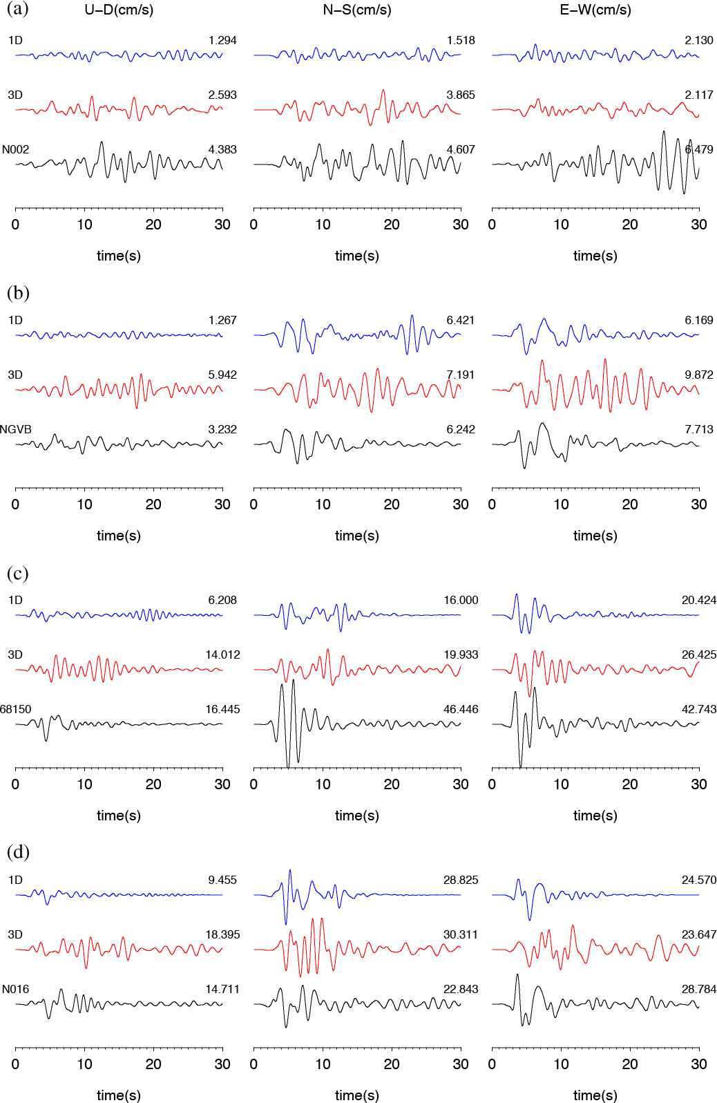
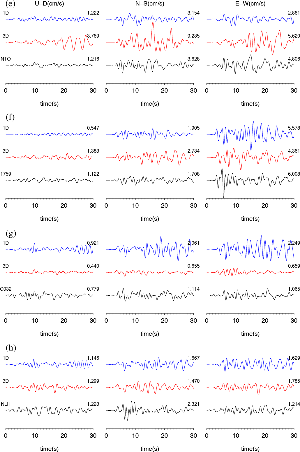
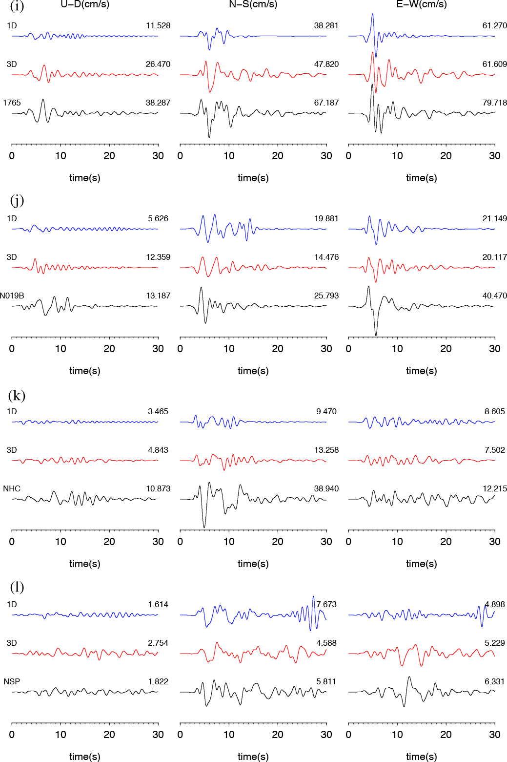
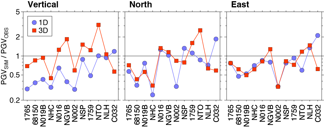
Figure S1 compares ground velocity waveforms simulated using 1D and 3D models with the recorded motions. All time series are filtered at f <1 Hz. For most sites, the 3D model does not have a dramatic effect on the simulated waveforms as compared with the 1D model. For sites located in the Napa Valley, where sediment depths are about 1.5 km (stations 68150, N016, and 1765), the 3D model predicts slightly larger amplitudes than the 1D model, although the simulated values are still lower than the observed (Fig. S1c,d,i). To more easily see the effect of the 3D model on peak motions, Figure S2 compares the ratio of simulated PGV for each component to the observed PGV for both the 1D and 3D models. The strongest systematic effect with the 3D model is an increase in the peak amplitudes of the vertical component motions by about a factor of 2 for nearly all the sites. The 3D model affects the amplitudes of the horizontal motions much less than it does the vertical motions, although there is some correlation with geology. For example, the horizontal motions at basin sites such as 68150 and 1765 are amplified relative to 1D, whereas nonbasin sites such as N019B and NSP are deamplified. At this point, the work with the 3D model is still preliminary. Further analysis of the model using smaller events (such as aftershocks) and including recordings from temporary arrays deployed after the mainshock will likely lead to improvements in the 3D velocity structure.
Because different reports indicate variation up to about 2 km for the mainshock epicenter, it is worthwhile to estimate the effect of such variation on the finite-fault inversion. In our analysis, the epicenter is used to constrain the dip of the southern fault segment, S3. For this test, we placed the epicenter beneath the mapped surface trace of the fault and assumed a vertical dip for the southern segment. This epicenter is very close to that determined by double-difference relocation (Hardebeck and Shelley, 2014). All other inversion parameters are the same as used for the preferred kinematic rupture model. The map view of the fault planes and resulting slip model are shown in Figure S3, along with the corresponding waveform fits. The slip distribution is quite similar to the inversion result presented in the main text, although the overall waveform fits are slightly worse than the preferred model (e.g., the north–south component for station NGVB). Our test demonstrates the relatively small sensitivity of the finite-fault inversion to the dip angle of the southern segment and, by extension, the epicenter location, given the variation between different catalogs. This is mainly due to the fact that the coseismic slip amplitude on the southern segment is relatively small, with most of the strong-motion energy coming from the shallow rupture on the northern segment.
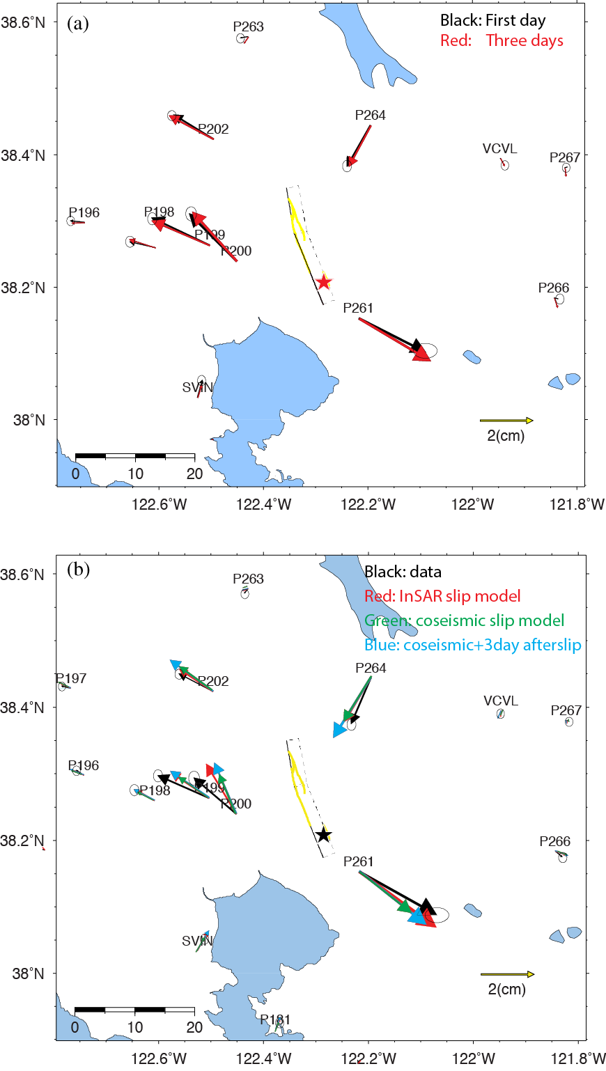
Continuous Global Positioning System (GPS) monitoring has been widely used to study the temporal variation of ground deformation. To investigate the presence of an afterslip signal on the near-fault stations, we use the GIPSY package to obtain the static offsets on these sites. The horizontal offsets were derived from the difference between time series observed one day before with those from one day and three days after the earthquake (Figure S4a). Our results show very similar values in these two data sets, indicating either the afterslip after one day of the earthquake is very small and/or the afterslip is very shallow and localized so that the signals can’t be seen on these stations.
To examine the impact of our after slip model on the broader static deformation field, we predict the static offsets at the nearby GPS stations using the coseismic slip model and a model that combines the coseismic slip and the first three days afterslip. As shown in Figure S4b, the coseismic slip model predicts a major portion of the static offsets, whereas the combined model predicts slightly larger offsets. Overall, the combined model produces very similar offsets to those from the InSAR slip model, and they both fit the data better than the coseismic slip model (Fig. S4b). Considering the very small difference observed between the first day observations and the three days observations (Fig. S4a), these results suggest most of the afterslip occurred within one day after the earthquake. However, because these GPS stations are greater than 10 km away from the epicenter, more data and modeling efforts are required to better resolve the spatial and temporal distribution of the afterslip.
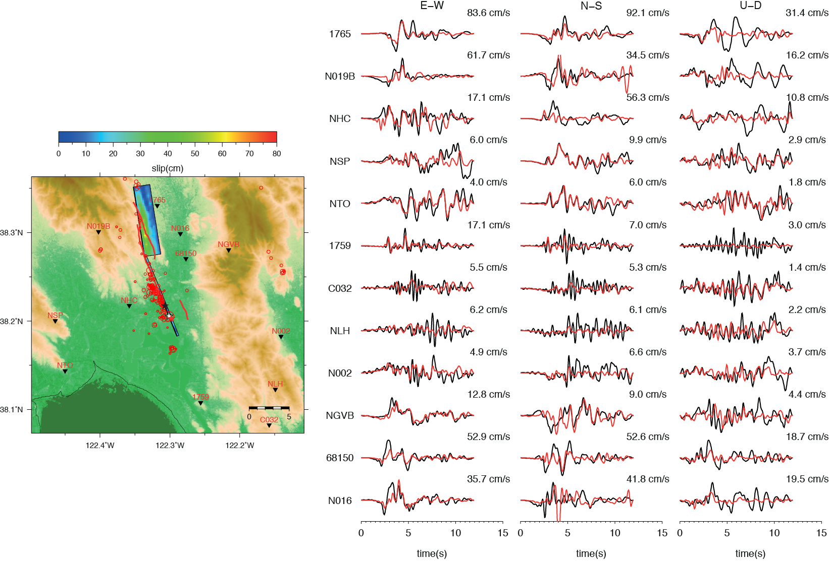
Figure S1: a–d, e–h, and i–l. Three-component velocity waveform comparisons for the 12 stations used in the inversion. The data are shown in black, the 1D synthetics in blue, and the 3D synthetic in red. All the waveforms are filtered to ≥1 Hz period. The 3D Bay Area 3D velocity model is used for the 3D simulation. The preferred kinematic slip model is used for the synthetics calculation. Note the difference between 1D and 3D synthetics in the vertical component. The data and synthetics are shown for (a–d) stations N002, NGVB, 68150, and N016; (e–h) stations NTO, 1759, C032, and NLH; and (i–l) stations 1765, NO198, NHC, and NSP.
Figure S2. Ratio of peak velocity for 1D (blue circles) and 3D (red squares) synthetics, with recorded data plotted for the 12 stations shown in Figure S1. The stations are ordered by decreasing observed peak velocity. Although horizontal-component ratios are similar between 3D and 1D, the 3D simulation systematically increases the amplitudes of the vertical motions by about a factor of 2–3.
Figure S3. Sensitivity test for the dip of segment S1. (Left) Locations of the fault segments (rectangles) that are used in the slip inversion of the earthquake. The upper bound of the fault is indicated by heavy solid lines. The dip angle of the first segment is 90°. The strike of the fault segment is chosen based on matching the surface rupture trace (red lines). The relocated seismicity in the first week is shown as open red circles, with the mainshock epicenter indicated by the white star (Hardebeck and Shelly, 2014). The red star indicates the epicenter used for this test. The black star is the 1D location shown for comparison. (Right) Observed and simulated velocity waveforms (f <3 Hz) for the 12 stations described in the main text.
Figure S4. (a) Comparison between horizontal GPS offsets derived from the difference between the time series one day before and one day (black) and three days (red) after the earthquake. The contribution of late afterslip (>1 day) is very small at these sites. (b) Prediction for the closest horizontal observed GPS offsets (black arrows) using various slip models, including the Interferometric Synthetic Aperture Radar (InSAR) slip model in Figure 5a of the main article (red), the coseismic slip model in Figure 3a of the main article (green), and a model that combines the coseismic slip and the first day afterslip (light blue). The GPS offsets were derived from the difference between GPS time series one day before and one day after the earthquake.
Kinematic_Slip_Model. Kinematic slip model of the Mw 6.1 South Napa earthquake.
Download: Kinematic_Slip_Model.zip (zipped plain text file; 6 KB]. Kinematic slip model of the Mw 6.1 South Napa earthquake.
Aagaard, B. T., R. W. Graves, D. P. Schwartz, D. A. Ponce, and R. W. Graymer. (2010). Ground-motion modeling of Hayward fault scenario earthquakes, Part I: Construction of the suite of scenarios, Bull. Seismol. Soc. Am. 100, no. 6, 2927–2944.
Brocher, T. A. (2005). Empirical relations between elastic wavespeeds and density in the Earth’s crust, Bull. Seismol. Soc. Am. 95, no. 6, 2081–2092.
Graves, R. W. (1996). Simulating seismic wave propagation in 3D elastic media using staggered-grid finite differences, Bull. Seismol. Soc. Am. 86, 1091–1106.
Hardebeck, J. L., and D. Shelly (2014). Aftershocks of the 2014 M 6 South Napa earthquake: Detection, location, and focal mechanisms, in 2014 Fall Meeting, American Geophysical Union, San Francisco, California, 14–19 December 2014, Abstract S33F-4927.
[ Back ]