This electronic supplement contains an installation guide, a short presentation on browsing, configuration, and evaluation test of the scisola software.
mysql-u root -p) and, in MySQL prompt, run source scisola.sql;.python scisola.py.Figures S1–S17 contain screen shots of each of the windows described here.
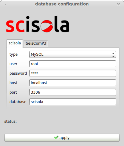
All settings and default values needed by the user to configure scisola are listed in Table S2.
To evaluate the quality of MT solutions produced by scisola, a dataset of 46 earthquakes that occurred in Greece from 24 January 2014 to 14 June 2014 was used (Table S3). Evaluation consists of comparing solutions provided by the automatic algorithm of scisola with the respective MT solutions that were calculated by the Geodynamics Institute, National Observatory of Athens (GI-NOA), in a manual way. Table S3 displays the information of the 46 MT solutions as calculated by GI-NOA and scisola.
Table S1. Description of the downloaded content.
Table S2. All settings and default values needed by the user to configure scisola.
Table S3. Results of the scisola and GI-NOA evaluations of the 46 MT solutions earthquakes that occurred in Greece from 24 January 2014 (2014-01-02) to 14 June 2014 (2014-06-25). The first row of the table contains the description for each column, the scisola results columns are preceded with an “A” in the header (e.g., AMw), and the last three columns contain the differences in magnitude, centroid depth, and focal mechanism determination (see main article for details).
Figure S1. Login window. By executing scisola, the Login prompt window will appear.
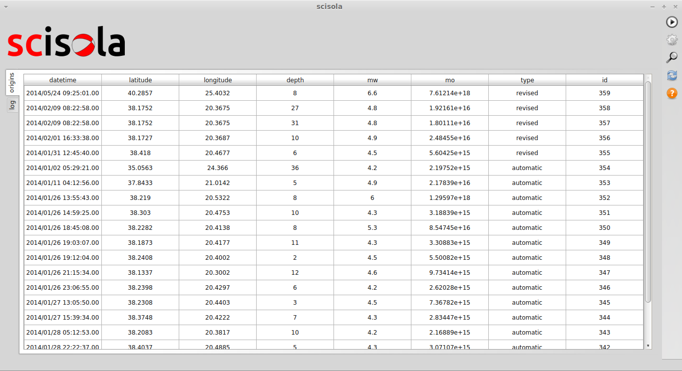
Figure S2. Main window. After successful login, the Main window will appear. It contains two tabs (origins, log) and the buttons area. the figure shows the origins tab.
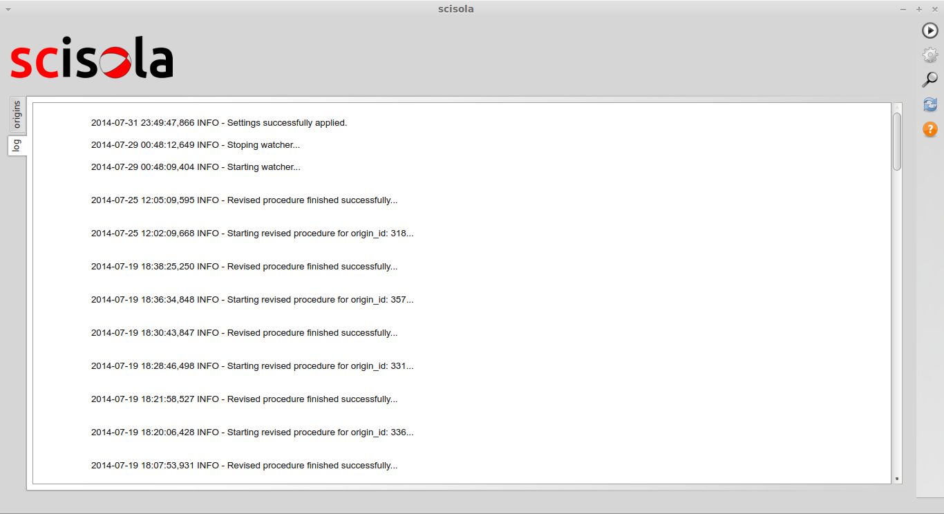
Figure S3. Main window. After the successful login, the Main window will appear. It contains two tabs (origins, log) and the buttons area. The figure shows the log tab.
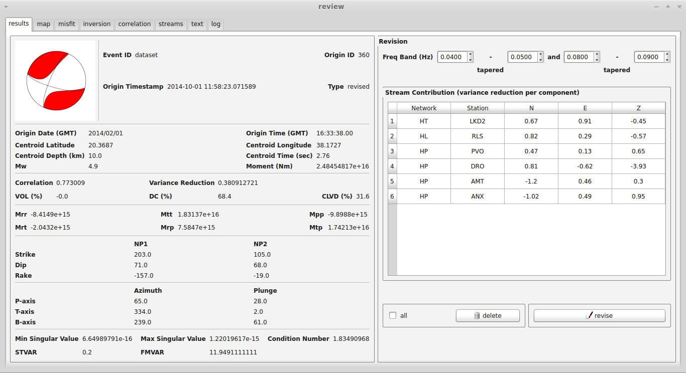
Figure S4. Inspection/Review window (review tab). By double clicking on an MT calculation (Figure S2), the user will be transferred to the Inspection/Review window. The first tab (results) contains the solution’s information, such as strike, dip, rake, correlation of the solution, and more, and it contains a revision panel where the user can change the inversion frequencies of the calculation or remove a stream (the number on each stream represents the variance reduction). This is a measure of the match between real and synthetic seismograms; for a detailed explanation see Křížová et al. (2013).
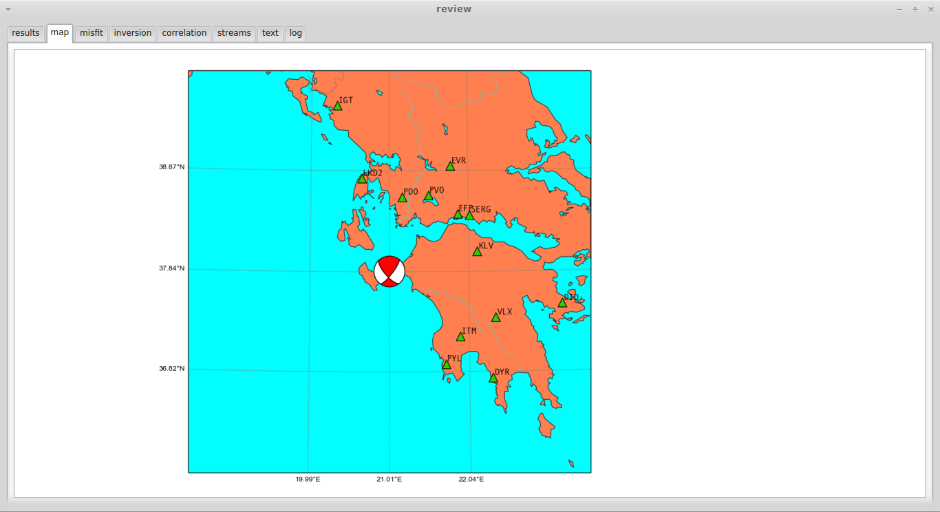
Figure S5. Inspection/Review window. The second tab (map) displays the generated map that contains the focal mechanism of the solution and the location of the stations contributing to the inversion.
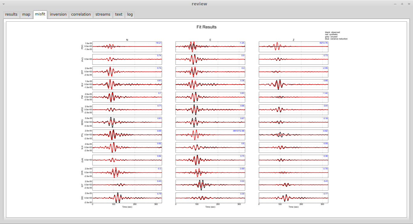
Figure S6. Inspection/Review window. The third tab (misfit) shows the misfit plot between the observed and synthetic waveforms.
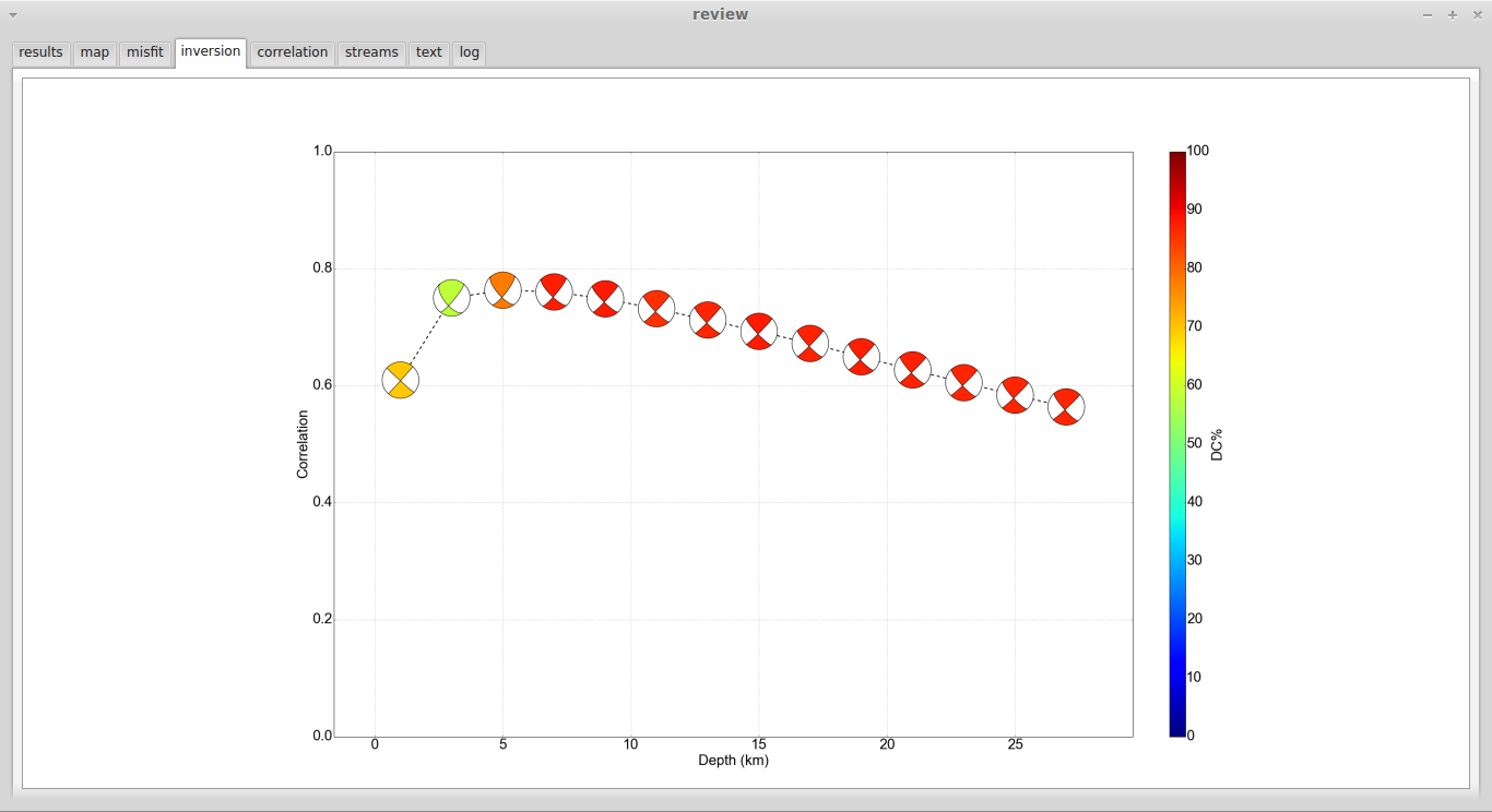
Figure S7. Inspection/Review window. The fourth tab (inversion) displays the generated plot containing the best focal mechanisms for each depth based on the correlation metric (i.e., the “best” solution is the solution with the highest correlation).
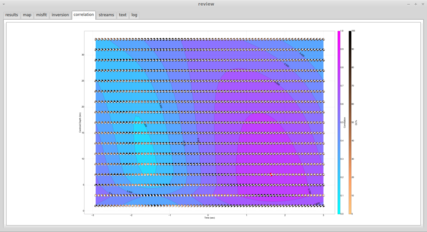
Figure S8. Inspection/Review window. The fifth tab (correlation) displays the generated plot containing all the focal mechanisms for each depth and for each time step before and after the origin time.
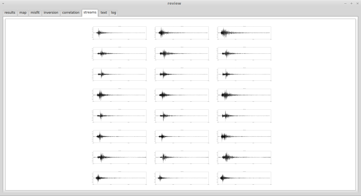
Figure S9. Inspection/Review window. The sixth tab (streams) shows the created plot that contains the streams contributing to the inversion.
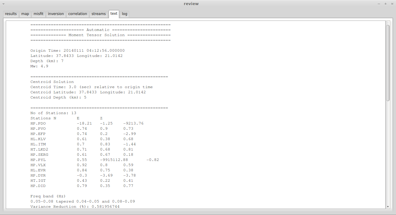
Figure S10. Inspection/Review window. The seventh tab (text) provides information about the MT solution in ASCII format, which is suitable for distribution over the Web. The number next to each stream is the variance reduction.
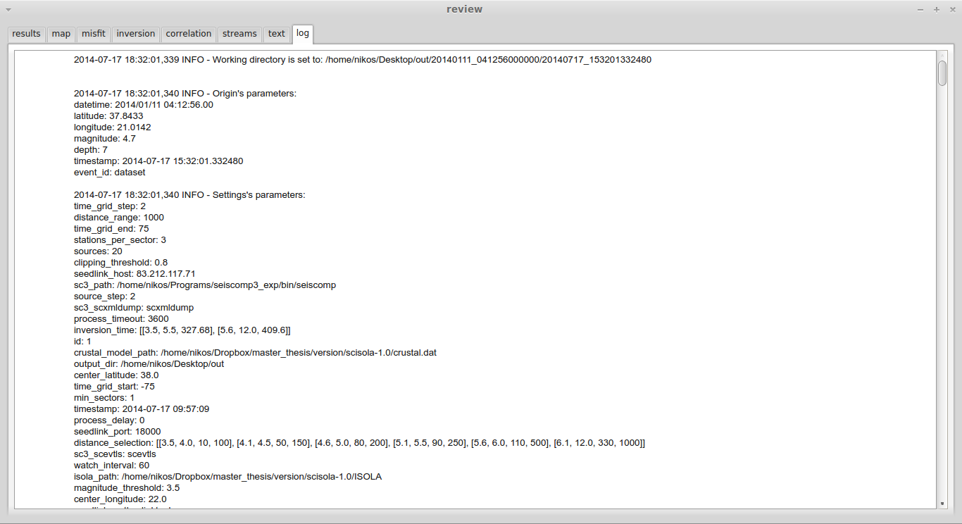
Figure S11. Inspection/Review window. The eighth tab (log) provides a log file containing the process information throughout the entire computation.
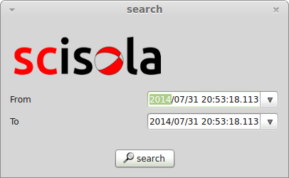
Figure S12. Search window. The third button pops up a Search window so that the user can search through previous MT calculations according to date–time range.
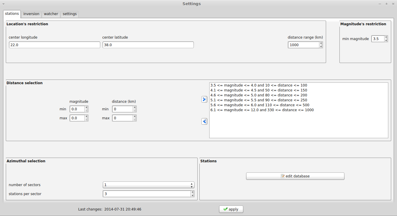
Figure S13. Settings window. The Settings window consists of four tabs. The first tab (stations) displays those settings that are relevant to station selection.
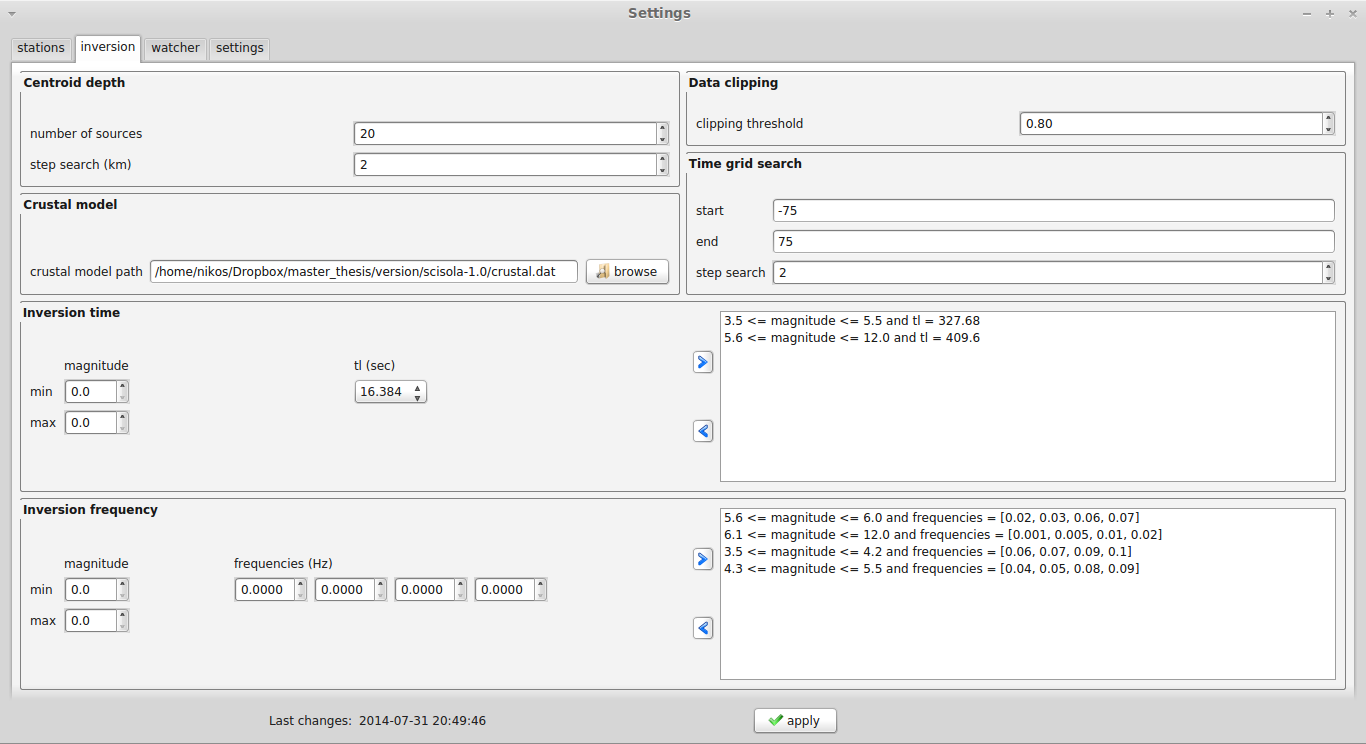
Figure S14. Settings window. The second tab (inversion) displays those settings that are relevant to the inversion procedure. The user must specify (a) the grid step for the centroid depth search, (b) the crustal model, (c) rules that connect the time length (tl, in seconds; fixed values) that will be used during inversion with the magnitude, (d) rules that connect the frequency band of the inversion with the magnitude, (e) a clipping threshold for waveforms (e.g., 0.80 means that if the recorded amplitude exceeds 80% of the theoretical maximum amplitude of the digitizer, the trace is considered as clipped), and (f) the centroid time grid search, start, step, and end relative to origin time. Units are given in dt, which is defined as tl/8192 (see Sokos and Zahradnik, 2008, for details).
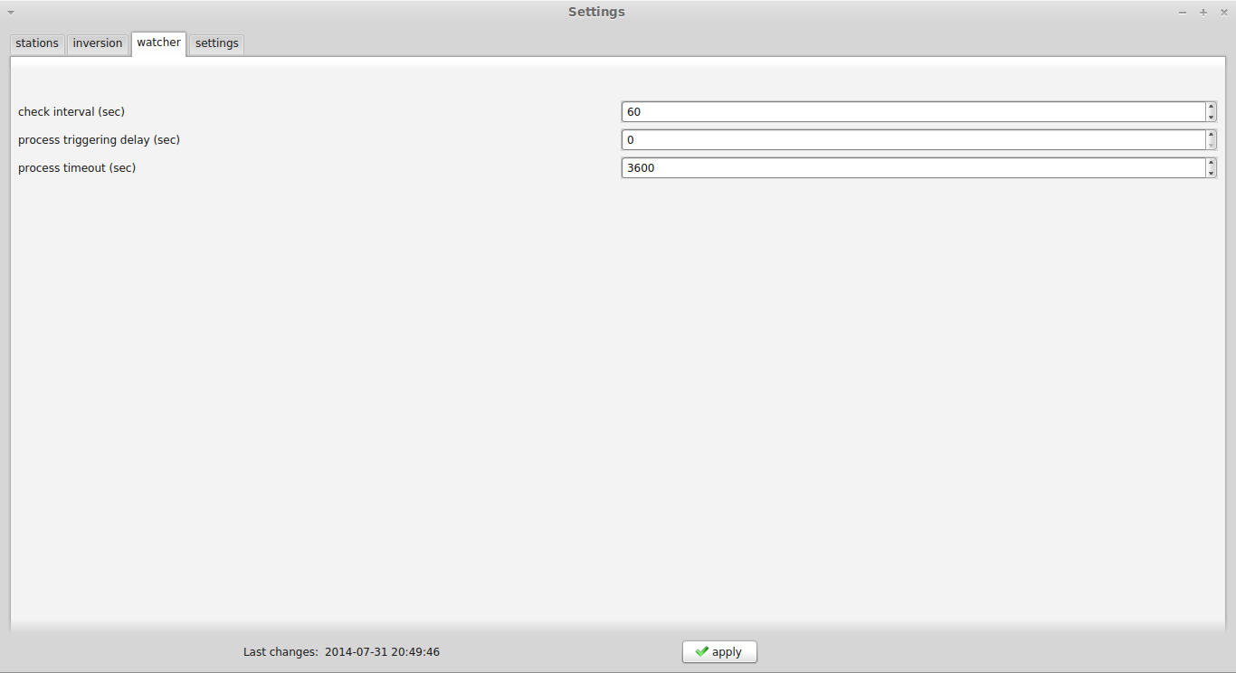
Figure S15. Settings window. The third tab (watcher) displays those settings that are relevant to the configuration of the watcher module.
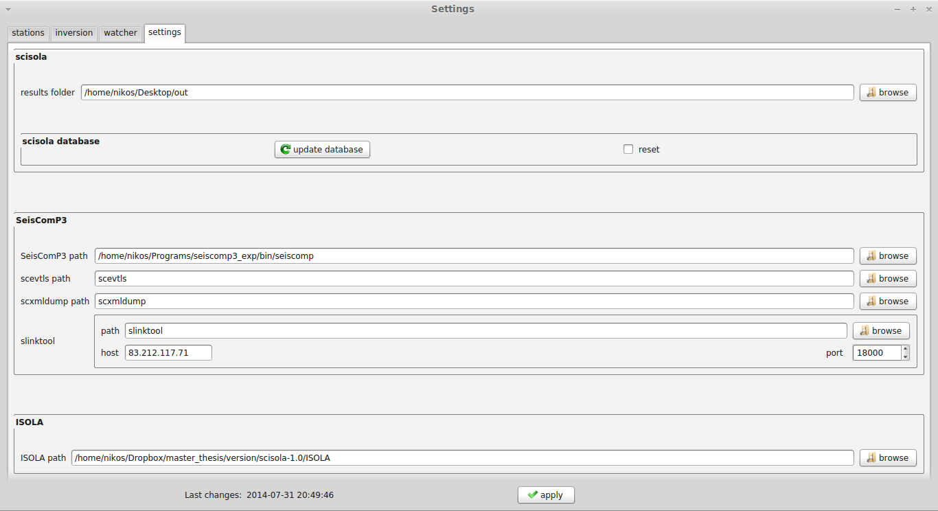
Figure S16. Settings window. The fourth tab (settings) displays more general settings of scisola.
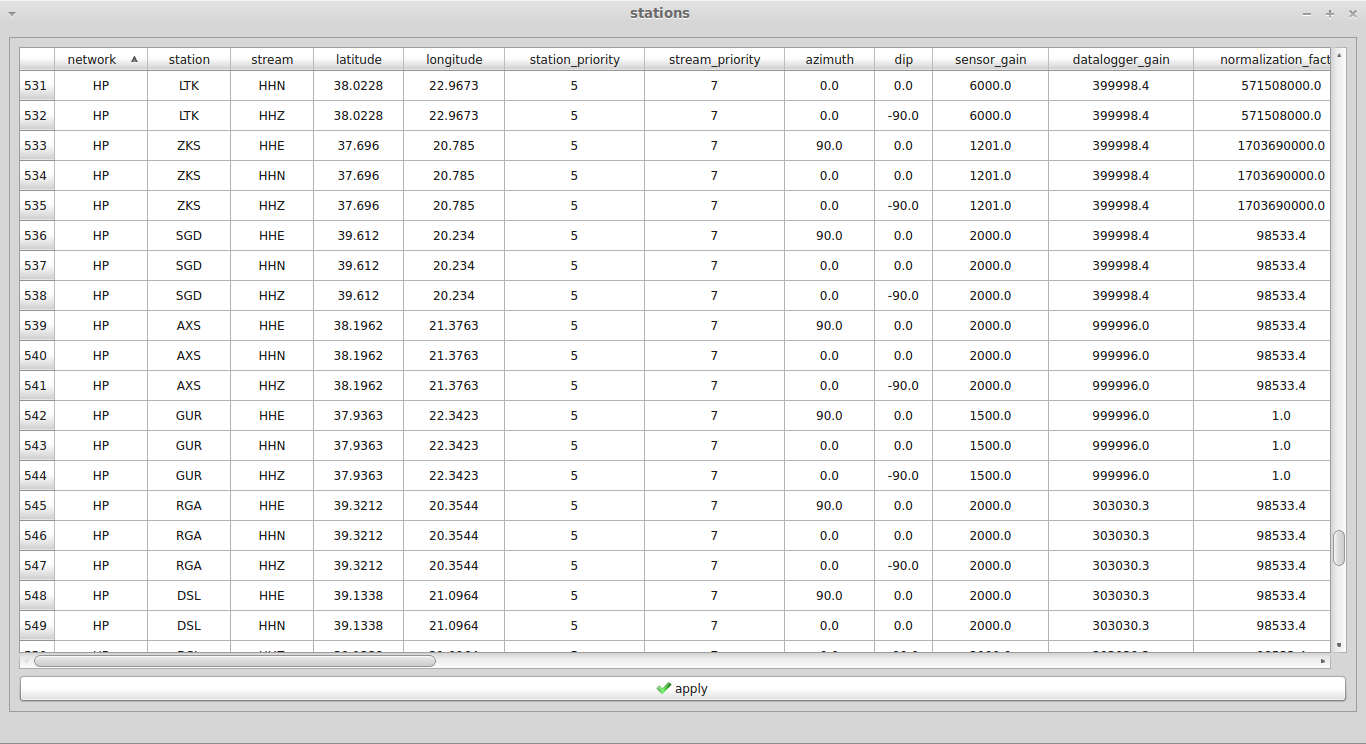
Figure S17. Stations window. By clicking on “edit database,” at the stations tab of the Settings window, a Stations window will appear that contains the stored information of all streams imported to scisola. The user can manually change the values for any stream. The possible values the user can alter are latitude, longitude, station priority, stream priority, azimuth, dip, sensor gain, datalogger gain, normalization factor, number of zeros, zeros content, number of poles, and poles content. By setting the station/stream priority to zero, the user can eliminate stations or streams from the inversion, thus taking into account technical problems in a station or stream. Station/stream priority is checked during the station selection procedure. By default, the value of stream priority is 7 for high gain seismometers (H), 6 for low gain seismometers (L), and 5 for any other case (e.g., accelerometers).
Scisola is available from the github repository (https://github.com/nikosT/scisola; last accessed October 2015).
Křížová, D., J. Zahradník, and A. Kiratzi (2013). Resolvability of isotropic component in regional seismic moment tensor inversion, Bull. Seismol. Soc. Am. 103, 2460–2473.
Sokos, E., and J. Zahradník (2013). Evaluating centroid-moment-tensor uncertainty in the new version of ISOLA software, Seismol. Res. Lett. 84, 656–665.
Sokos, E. N., and J. Zahradník (2008). ISOLA a FORTRAN code and a MATLAB GUI to perform multiple-point source inversion of seismic data, Comp. Geosci. 34, no. 8, 967–977, doi: 10.1016/j.cageo.2007.07.005.
[ Back ]