This electronic supplement provides details on the moment tensor (MT) inversion procedure and a test MT inversion with synthetic data, and contains results of simulated annealing MT inversion using a synthetic dataset and a table of amplitude correction coefficients for each station used for the MT inversion.
Prior to all MT inversions, we empirically determine amplitude correction factors for used seismic stations. We collect 51 suitable earthquakes with epicentral distances of 5000–8000 km from the explosion site, occurring 1–360 days before the January 2016 explosion, with magnitude between Mw 6.5 and 7.5. Synthetic seismograms are computed using the MT solution by Global Centroid Moment Tensor (Global CMT) and the IASP91 velocity model. Vertical synthetic displacements are compared with real data in the 0.01–0.05 Hz frequency range, for a time window of 200 s duration, starting 50 s before the P-wave arrival. Only waveforms with a high cross-correlation coefficient of more than 0.8 are considered. Synthetic and real data are aligned and the scaling factor derived. The final scaling coefficients for each station (Table S1) are found as the mean for the 51 different earthquakes.
We employ a stochastic global optimization procedure to find an ensemble of source models with acceptable data fit. The optimization procedure investigates simultaneously a multidimensional space of 10 source parameters: centroid time, latitude, longitude, depth, and six independent MT components. These parameters vary within predefined realistic intervals. Misfits (L2 norm) are computed separately for each trace and used to simulate different station configurations using a bootstrap approach. We fit amplitude spectra of radial, vertical, and transversal full waveforms (below 1200 km epicentral distance) and displacement waveforms (below 600 km) in the 0.02–0.04 Hz frequency range. During a training period (1000 iterations), source models are chosen randomly; in a second stage (300,000 iterations), the algorithm iteratively computes the multivariate covariance from the best 100 solutions, derives the multivariate distribution parameters, and produces random new models accordingly. The search of new models becomes increasingly sharper.
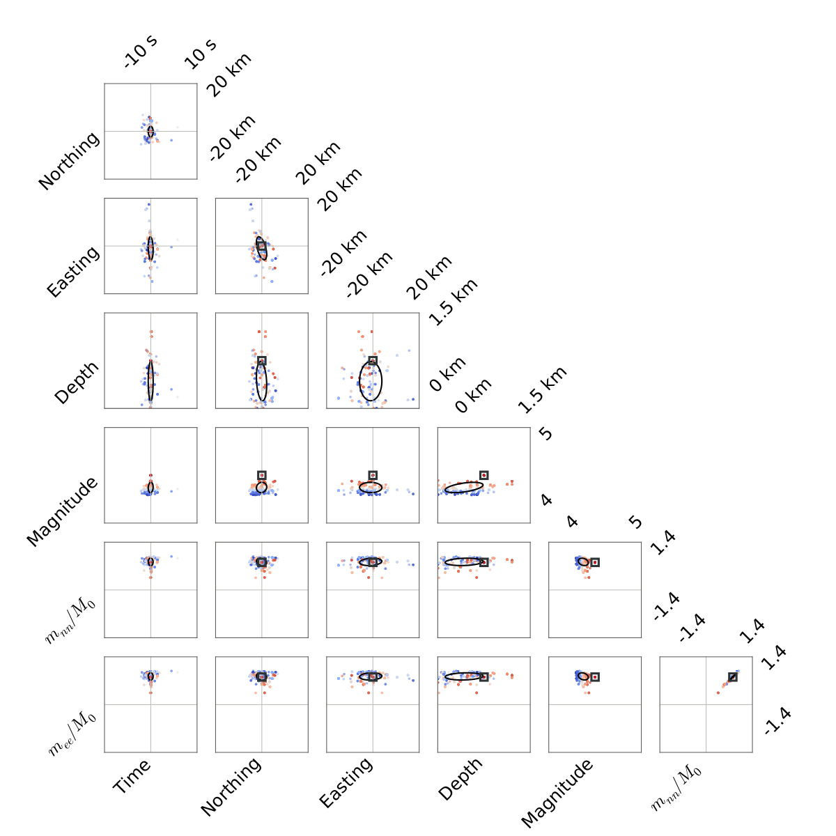
We demonstrate the intrinsic ambiguity that affects the procedure of full-waveform MT inversion for a shallow explosion source, even with a known velocity model and noise-free data. Full-waveform displacement synthetic data correspond to an isotropic source at 129.07° E, 41.31° N, depth 750 m, and moment magnitude 4.5. The adopted velocity model (MDJ2) and stations configurations are equivalent to those used for the inversion of the 2016 explosion. We use the simulated annealing MT inversion algorithm. Figures S1, S2, and S3 provide a summary of the inversion results, considering 3000 best solutions. For the synthetic test, the range of best solutions is obtained both considering different MT solutions well fitting a certain station distribution, and also simulating different station distributions (out of the existing dataset) within a bootstrap approach. Solutions are plotted for all pairs of considered source parameters.
Table S1. Amplitude correction coefficients for each station used for the MT inversion.
Figure S1. Results of the simulated annealing MT inversion using a synthetic dataset for an isotropic source, showing the first panel of comparison of source parameters pairs (the figure is complemented for other parameters pairs by Figs. S2 and S3). Results are plotted for the best 3000 solutions. The reference input source model is shown by a black square. Different solutions (dots) are colored according to the moment magnitude (blue to red, for increasing magnitude). Trade-offs are depicted corresponding to off-axis–oriented standard deviation ellipses (black line ellipses).
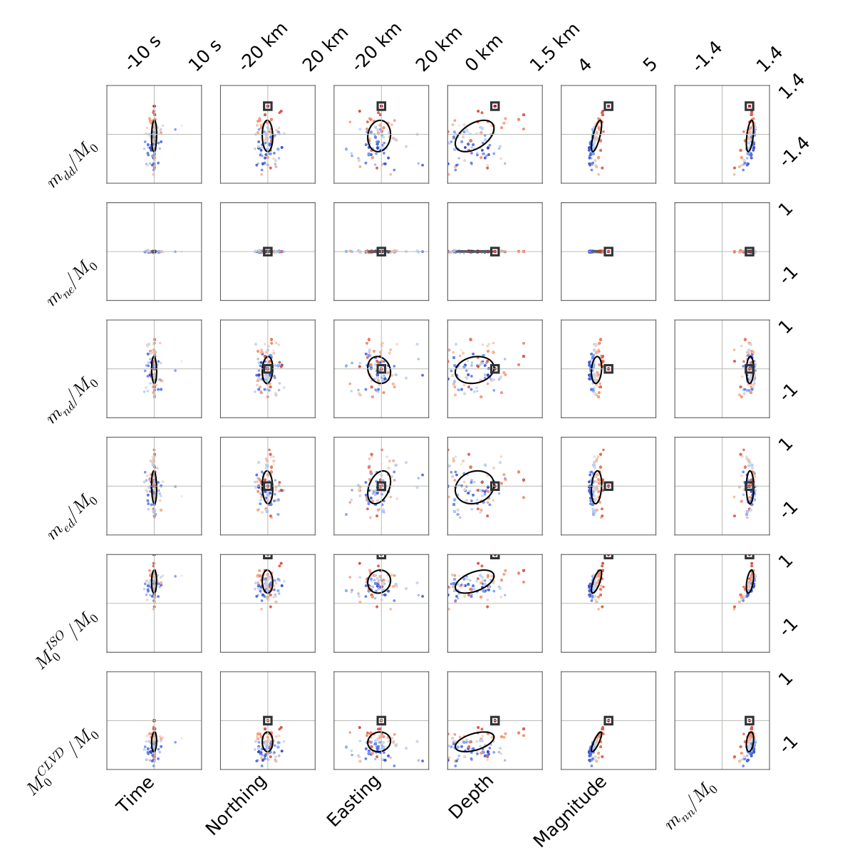
Figure S2. Results of the simulated annealing MT inversion using a synthetic dataset for an isotropic source, showing a second panel of comparison of source parameters pairs. The graphical layout is the same as Figure S1.
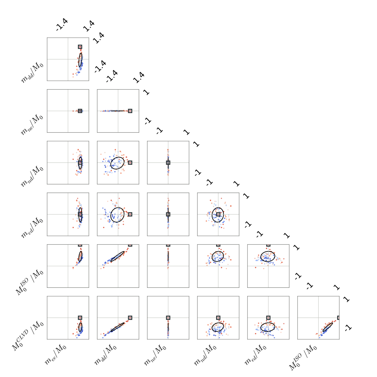
Figure S3. Results of the simulated annealing MT inversion using a synthetic dataset for an isotropic source, showing a third panel of comparison of source parameters pairs. The graphical layout is the same as Figure S1.
[ Back ]